Choose L1 regularization when an intentionally sparse model is part of the goal. Its penalty can drive some coefficients exactly to zero, allowing a model to use fewer features. Choose L2 when you want continuous coefficient shrinkage without making exact-zero feature selection the objective. In either case, select the penalty strength with validation data and confirm that your estimator and solver support the penalty you requested.
Neither method is universally more accurate. The right choice depends on whether sparsity, smooth shrinkage, interpretability, prediction quality, computational constraints, or implementation compatibility matters most for your task.

As an Amazon Associate I earn from qualifying purchases.
What L1 and L2 regularization change
Regularization adds a penalty for large coefficients to the model’s loss function. Instead of minimizing prediction error alone, the estimator minimizes prediction error plus a term that discourages coefficient magnitude. This limits overfitting and makes the fitted model less dependent on any one training sample.
The Tool Desk
Outbyte Driver Updater FREEScan for outdated or missing drivers - takes under a minuteDriver Scan →Outbyte PC Repair FREERepair Windows errors before they cause bigger problemsFix Now →For a linear model with coefficients w, a common objective can be written as:
#1 Best Overall

- [Ultra-Lightweight Ear Buds Designed for Small Ears] Each earbud weighs only 3.7g and features a compact, ergonomic in-ear design made especially for small ears. Secure, low-profile, and comfortable for workouts, all-day wear or overnight sleeping.The ultra-slim profile sits flush in your ear with no hard edges poking or rubbing, so you can even sleep on your side without discomfort.
- [Immersive Stereo Sound with TOZO OrigX Technology] TOZO OrigX tuning delivers clear vocals, balanced mids, and natural stereo sound for music, podcasts, and videos.
- [Long Battery Life for Daily Use] Get up to 7 hours of playtime on a single charge, with up to 32 hours total using the charging case—ideal for workdays, commuting, and extended listening sessions.
- [Bluetooth 5.3 & Stable Connection] Bluetooth 5.3 provides fast pairing, stable wireless performance, and reduced dropouts as you move around home or office.
- [Deep Bass with Clear Vocals] High-performance drivers produce punchy bass while keeping vocals clean and detailed for everyday listening.
loss(data, w) + alpha × penalty(w)The difference between L1 and L2 is the shape of that penalty:
- L1:
||w||₁ = |w₁| + |w₂| + … + |wₚ| - L2:
||w||₂² = w₁² + w₂² + … + wₚ²
L1 creates a sharp corner at zero. During optimization, that geometry makes an exact zero a natural solution for some coefficients. The scikit-learn User Guide describes this directly: “The Lasso is a linear model that estimates sparse coefficients, i.e., it is able to set coefficients exactly to zero.” L2 has a smooth penalty. It normally reduces coefficients toward zero without turning them into exact zeros.
Different libraries place constants and scaling factors in their objectives, so the same numeric value is not automatically equivalent across estimators. Treat alpha, lambda, and C as estimator-specific parameters rather than interchangeable names.
PC Slower Than It Used to Be?
A free scan shows the junk files, broken settings and background clutter dragging Windows down - then fixes them in one click.Free scan · Windows 10 & 11Outdated Drivers Are Slowing You Down
One free scan finds every outdated or missing driver and matches the right update for your exact hardware.Free scan · exact hardware matchQuick decision: which penalty fits your objective?
| Decision axis | L1 / Lasso | L2 / Ridge |
|---|---|---|
| Coefficient effect | Can set some coefficients exactly to zero | Shrinks coefficients through a squared-magnitude penalty |
| Best fit for | A deliberately sparse model or an embedded feature-selection objective | Continuous shrinkage when exact-zero selection is not required |
| Interpretation | Produces a smaller active feature set, but selected features are not automatically stable or causal | Keeps all eligible features in the model while reducing their influence |
| Tuning | Choose penalty strength against the task’s validation objective | Choose penalty strength against the task’s validation objective |
| Implementation concern | Estimator and solver must support L1 | Estimator and solver must support L2 |
Use the table as a starting rule, not a performance ranking. Compare both penalties with the same data splits, preprocessing, and metric when prediction quality is the deciding factor.
Choose L1 when sparsity is a requirement
When a compact feature set is useful
L1 is attractive when you need a model that actively discards some input variables. A coefficient of exactly zero means that feature does not contribute to that fitted model’s linear prediction. The resulting active set can simplify scoring, reduce the number of measurements required at inference time, or make a high-dimensional model easier to inspect.
This is an objective about representation, not a promise about scientific truth. A nonzero coefficient is not proof that a feature causes the outcome, and a zero coefficient is not proof that the underlying phenomenon is irrelevant. The selected set can change when the training sample, preprocessing, or validation split changes.
When the number of features is large relative to observations
In a wide design matrix, a sparse solution can be operationally useful because it limits the number of variables carried into deployment. L1 gives the optimizer a mechanism for removing variables as the penalty increases. You still need to validate the resulting model on data that represents the intended use; sparsity alone does not establish generalization.
What’s actually slowing this PC down?
Pick the symptom - the matching free tool is one click away.
Rank #2

- 【IP68 Waterproof Multifunctinal Smart Watch】Torjalph fitness activity tracker smart watch is IP68 waterproof technology ,you can wear it when swimming,handwashing,it's rain-proof which means that you perform multiple exercise modes outside without worrying about sweat or rain corroding your fitness smart watch,and this watch equipped with a 230 mAh large capacity battery magnetic charging ,and this sports activity tracker watch can be used 5-7 days If fully charged.
- 【Larger 1.83'' Full Screen Watch & Multi-dial Selection】1.83 inch full HD color touch screen smart watch for men / women provides excellent 240*284 resolution image quality ,This Bluetooth smart watch offers a better touch experience and remarkable immersion and ,more than 200 watch faces for you to choose from App"Da Fit ", you can change the dial style according to your mood to wear keeping the world on your wrist
- 【Accurate Activity Tracker Smart Watch 】sports watch activity tracker uses sweat and dust resistant breathable silicone strap, our Fitness Tracker Smart Watch for Android iOS Phones supports 12 sports modes,walking,running,bicycle,swimming,badminton,basketball,football,rope skipping. This bluetooth calls smart watch for men women is lightweight and stylish, bringing more convenient and relaxing sports experience while also providing more protection.
- 【Your 24 Hour Personal Daily Health Monitor】Fitness watch for women men full touch screen IP67 waterproof bluetooth smartwatch for Android iOS Phones with heart rate blood pressure monitor multifunction Andriod smart watch with steps counter sleep monitor sports fitness watch, monitoring blood oxygen saturation allows you to understand your physical condition in real time to track fitness progress ,to know your health status in time.
- 【More Functions Bluetooth Call Smart Watch】This fitness activity smart watch full screen for iPhone and Android phones includes a bunch of new features including:The bluetooth smart watch can hang up the phone, receive and display WhatsAPP /Text /Facebook /Twitter /Messenger reminder.Support sedentary reminder, alarm clock, stopwatch, timer,weather information,music control, remote camera control compatible with Android 5.0 and above or iOS 9.0 and above smartphones.
When feature selection must happen inside the modeling workflow
L1 performs selection while fitting the predictive model. That can be preferable to ranking features once with a separate univariate test, provided the entire selection process is fitted only on the training portion of each validation split. If you select features on the full dataset before cross-validation, information from validation folds leaks into training and can make the reported score optimistic.
What L1 does not guarantee
- It does not guarantee that the selected variables remain the same across samples.
- It does not guarantee that every genuinely useful variable survives the penalty.
- It does not guarantee better predictive accuracy than L2.
- It does not remove the need to scale numeric features or to validate the complete pipeline.
If the identity of selected features is itself a deliverable, measure its reproducibility under the resampling scheme and data conditions you expect in production. The official documentation defining Lasso’s sparsity does not establish a universal feature-selection stability guarantee.
Choose L2 when smooth shrinkage is the priority
When every feature may contribute
L2 is the usual Ridge-style choice when you want to reduce coefficient magnitudes but do not want the regularizer to make exact-zero selection the central goal. Every feature can retain a small contribution, which is useful when many weak signals collectively matter.
When you want a smooth optimization problem
The squared L2 penalty is differentiable, making it a natural fit for many optimization methods. In practical terms, L2 often offers a straightforward baseline for linear and generalized linear models. The relevant estimator still determines which solvers and penalty options are available.
Free tools Windows power users keep installed
One-click scans. No signup required.
When deleting variables would be undesirable
In some workflows, downstream systems expect a fixed feature schema, or domain experts prefer to retain all measured variables while moderating their influence. L2 preserves that schema. It can also avoid turning a small coefficient into an all-or-nothing decision when the cost of dropping a variable is high.
What L2 does not provide
L2 shrinkage is not feature selection. A coefficient that is merely small is still present, and a model with all coefficients retained may require the same measurements and processing as an unregularized model. If your explicit requirement is an exact-zero active set, evaluate L1 or a mixed penalty instead.
Scaling is part of the penalty decision
Regularization acts on coefficient magnitudes, so feature units affect the result. Suppose one variable is measured in dollars and another in thousands of dollars. Their coefficients can have very different numerical scales even when their predictive contribution is comparable. Applying the same penalty to those raw coefficients therefore penalizes the variables unevenly.
Rank #3
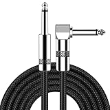
- [Low Noise High Fidelity] New bee guitar cord with 22AWG oxygen-free-copper center conductors provides enhanced signal transfer, the PVC insulation material and the high-density stranded copper double shield provide noise rejection for quiet operation
- [Ideal for Choice] New bee 1/4 straight and right angle metal connectors, ensures a secure connection in any instrument, pedal, or amp jack. L shape great fro on stage guitar stands
- [Wide Compatible] Suitable for mixer, power amplifier, microphone, effector, decoder, equalizer, electoronic organ, electric guitar, electric bass and other electronic equipments. Widely used in the installation of smart home, karaoke speaker, professional stage audio, etc
- [Easy Disassemble] Making incidental repairs quick and easy! Very nice, flexible cable
- [Dont Hesite to Order] 24 hours customer services and professional technology team are standing by
For numeric predictors, fit a scaler on each training fold and apply that fitted transformation to its validation or test data. Keep the transformation and estimator in one pipeline so that cross-validation cannot use information from held-out rows. Decide separately how to handle binary indicators, sparse matrices, missing values, and categorical encodings; the correct preprocessing depends on the data representation and estimator.
Quick wins for a faster PC:
Repair Windows errors before they cause bigger problemsFix Now →Fix the driver behind crashes, sound loss and screen glitchesFind Drivers →Clear out junk files and repair common Windows errorsFree Scan →Do not standardize the target merely because predictors are standardized. Target transformation is a separate modeling decision that must be reversed correctly when predictions are reported in the original units.
How to tune the penalty strength
1. Define the validation objective first
Choose the metric that represents the decision you will make. For regression, that could be a loss based on absolute or squared error; for classification, it could be accuracy, a ranking metric, log loss, or a cost-sensitive measure. A penalty value that is best for one metric is not necessarily best for another.
2. Build preprocessing into the estimator
Use a pipeline that fits scaling, encoding, imputation, and the regularized estimator inside each training fold. This prevents preprocessing statistics and feature-selection decisions from leaking across folds.
3. Search a logarithmic range
Penalty strengths commonly span several orders of magnitude. Search a geometric sequence rather than a short linear list. Include a value close to no regularization only when the estimator and numerical behavior make that comparison meaningful. The optimal range depends on sample size, feature scale, noise, and the estimator’s objective.
Recommended Free Tools
4. Use cross-validation on the training data
For each candidate strength, fit on the inner training folds and score on the corresponding validation fold. Select the value using the metric and direction you defined. Keep a final test set untouched until the model and penalty have been chosen.
5. Refit once and report the complete procedure
After selecting the hyperparameter, refit the pipeline on the data allowed for final training, then evaluate once on the held-out test set. Record the preprocessing, estimator, penalty, search range, split strategy, random seed where applicable, and metric so another person can reproduce the result.
Rank #4

- Digital Family Calendar: BSIMB digital calendar wall touch screen puts an end to your chaotic life. Designed for busy families, the digital calendar keeps you organised and in step with your family. Assign different colours and tasks to each family member to make family scheduling easier and more intuitive.
- Easy Setup and Auto-Sync: Plug in, connect to WLAN and auto-syn your electric calendar in minutes. Digital wall calendar compatible with Google calendar, iCloud calendar, Outlook calendar, Cozi calendar and Yahoo calendar. Add events directly on the device or through the ecalendar app. Electronic calendar stays current whether you're at work or traveling—no manual updates needed.
- All-In-One Home Assistant: Smart calendar builds habits and encourage independence with personalised chores. Display daily meal plan to reduce the daily ‘What's for dinner?’ stress. To-do lists keep track of everything you want. Turning chores into valuable achievements with stars and rewards, making life easier and more enjoyable.
- Manage Anytime Anywhere: BSIMB electronic calendar for family stay connected with the powerful ecalendar app. Access and manage your digital wall calendar anytime, anywhere with free features like stars & rewards, photo screensaver, chore charts, meals plans, to-do lists etc. Electronic planner paid features like Magic Import tailor advanced tools for users with special needs.
- Stay in Touch with Loved Ones: Share photos or videos from your phone to electronic wall calendar with app, instantly update your life moment, and keep in touch with your family, especially those who are far away; you can also surprise your smart calendar digital wall by sending him a wish card; it's also great for keeping tech-illiterate elders in touch with the youngsters.
For Lasso, scikit-learn documents alpha as the parameter multiplying the L1 term. Its documentation also describes cross-validation tools for choosing alpha and information-criteria alternatives. Those tools still depend on the estimator’s objective and your data; do not copy an alpha value from another dataset as if it were universal.
Estimator parameters are not interchangeable
Parameter names can be misleading when moving between estimators. In scikit-learn’s LogisticRegression, C is an inverse regularization-strength parameter: larger C means weaker regularization, while smaller C means stronger regularization. In documented Lasso estimators, alpha directly scales the L1 term. A value such as alpha=1 cannot be translated mechanically into C=1.
Do these 3 things before closing this tab:
1Fix the driver behind crashes, sound loss and screen glitches2Repair Windows errors before they cause bigger problems3Scan for outdated or missing drivers - takes under a minuteRead the API documentation for the exact estimator and software version used by your project. Check the objective’s scaling conventions, default penalty, intercept treatment, class weighting, and whether the implementation normalizes or standardizes internally.
LogisticRegression solver compatibility in scikit-learn
The current scikit-learn LogisticRegression documentation surfaced for this topic lists penalty support by solver as follows. These are implementation details tied to that documentation version; verify them against the version installed in your project before copying a configuration.
| Solver | Documented penalty support | Practical implication |
|---|---|---|
lbfgs |
L2 or no penalty | Do not request L1 or Elastic Net |
newton-cg |
L2 or no penalty | Use an L2-compatible configuration |
newton-cholesky |
L2 or no penalty | Check version and memory requirements for your data shape |
sag |
L2 or no penalty | Use an L2-compatible configuration and scale features appropriately |
liblinear |
L1 or L2; not Elastic Net | Choose one of the two supported penalties; confirm multiclass behavior separately |
saga |
Supports Elastic Net | Use it when a mixed L1/L2 penalty is required, subject to the estimator’s other constraints |
A solver error is often a compatibility problem rather than evidence that the penalty is mathematically unsuitable. Check the solver–penalty matrix, the estimator version, and the data format before changing the model objective.
Independent reader supportYour contribution helps us test, update, and keep practical guides available for everyone.Elastic Net: when neither pure penalty is enough
Elastic Net combines L1 and L2 terms. One component encourages exact zeros; the other supplies continuous shrinkage. This is useful when you want a sparse model but do not want the behavior of a pure L1 penalty to determine the entire coefficient pattern.
Its two choices must both be tuned: the overall regularization strength and the mixture between L1 and L2. A model with a large L1 share behaves more like Lasso; a model with a large L2 share behaves more like Ridge. Use the same leakage-safe pipeline and validation design as for either pure penalty.
Elastic Net is not universally superior. It adds a hyperparameter and therefore a larger search space. Use it when the mixed objective addresses a real modeling requirement, not simply because it offers more settings.
A practical comparison workflow
For a regression problem
- Separate predictors, target, and a final test set before model selection.
- Identify numeric, categorical, indicator, and missing-value columns.
- Construct a pipeline that performs the required preprocessing and then fits a Lasso, Ridge, and optionally Elastic Net estimator.
- Search each estimator’s own strength parameter on a logarithmic grid.
- Use identical folds and the same regression metric for every candidate.
- Inspect both the cross-validation score and the coefficient pattern. If sparsity is required, check how many coefficients are exactly zero after refitting.
- Choose the simplest model that satisfies the predictive and operational requirements, then evaluate it once on the untouched test set.
For a classification problem
- Choose the classification metric and split strategy before tuning.
- Scale continuous predictors inside the cross-validation pipeline.
- For
LogisticRegression, choose a solver that supports the requested penalty and useCvalues that span weaker and stronger regularization. - Compare L1, L2, and Elastic Net only when the selected solver supports each configuration.
- For imbalanced classes, incorporate the intended class weights or resampling inside the training procedure and keep validation data representative of deployment.
- Evaluate probability calibration or decision-threshold behavior if the application uses probabilities or asymmetric costs.
The code shape below illustrates the separation between a pipeline, a parameter search, and estimator-specific parameters. Substitute values appropriate to your dataset and installed scikit-learn version.
Pipeline([("scale", StandardScaler()), ("model", LogisticRegression(...))])

# Tune model__C for LogisticRegression.
# Tune model__alpha for estimators that expose alpha.
# Do not assume these parameters have the same meaning.
Common failure modes and fixes
“My L1 model keeps every feature.”
Check whether the selected penalty is strong enough, whether the coefficients are being inspected before or after scaling, and whether numerical tolerances make very small values appear nonzero. Confirm that the estimator actually uses L1 and that the chosen solver supports it. If the validation objective favors a weak penalty, retaining many features may be the correct result.
“My L2 model has no zeros.”
That is expected. L2 shrinks coefficients but is not intended to perform exact-zero feature selection. If an explicit sparse representation is required, evaluate L1 or Elastic Net.
“The validation score changes sharply with the penalty.”
Expand the search range, inspect fold-to-fold variation, and verify that preprocessing is inside the pipeline. Large variation can indicate a small dataset, noisy metric, distribution differences between folds, or a model that is sensitive to the regularization regime. Use repeated or nested validation when the decision warrants a more stable estimate.
“The solver rejects my penalty.”
Read the estimator’s versioned documentation and select a compatible solver–penalty pair. In LogisticRegression, the documented support differs across lbfgs, newton-cg, newton-cholesky, sag, liblinear, and saga. Changing the solver can also change convergence behavior and computational cost, so retune rather than assuming the previous parameter remains optimal.
“The selected features change between folds.”
Do not interpret that instability as a software error. Refit under resampled training sets, quantify how often each feature is selected, and decide whether a stable feature list is truly required. If it is, consider whether L2 or a mixed penalty better matches the operational objective. The documentation establishing Lasso’s ability to create zeros does not promise stable selection under correlated or changing data.
“Training succeeds, but production performance falls.”
Audit the split strategy, feature availability at prediction time, preprocessing fit boundaries, target leakage, and distribution shift. Regularization controls coefficient magnitude; it cannot correct a deployment pipeline that uses information unavailable at inference.
How to make the final choice
Start with the requirement that cannot be compromised. If the model must use a small subset of variables, put L1 or Elastic Net in the candidate set and evaluate selection reproducibility as well as predictive score. If all measured variables remain eligible and you want controlled, continuous shrinkage, make L2 the baseline. If neither objective dominates, compare L1 and L2 under identical validation conditions and let the task metric, operational constraints, and implementation support decide.
Document the chosen penalty, estimator, solver, strength parameter, preprocessing, data split, and validation metric. That record is essential because regularization settings are properties of a complete modeling pipeline, not universal constants that can be transferred unchanged to another dataset.
Quick Recap
Product prices and availability are accurate as of the date/time indicated and are subject to change. Any price and availability information displayed on Amazon at the time of purchase will apply.




