Recommended Free Tools
The clearest spin-ice visualization uses three synchronized views: a temperature–field phase map, a real-space map of vertex charges and flipped-spin strings, and a reciprocal-space structure-factor map. The first shows where thermodynamic or magnetic behavior changes; the second shows ice-rule violations directly; the third reveals long-range Coulomb-phase correlations through features such as pinch points.
To make those views trustworthy, define the spin convention and observables before plotting, equilibrate every temperature–field point with an appropriate Monte Carlo method, retain configuration snapshots, and attach uncertainty estimates from independent runs. Keep the same parameter point, field direction, lattice size and sign convention across all panels.

As an Amazon Associate I earn from qualifying purchases.
What a spin-ice phase diagram and defect map should show
Spin ice consists of frustrated magnetic moments constrained by corner-sharing tetrahedra in bulk pyrochlores or by patterned nanomagnets in artificial lattices. Each local tetrahedron or vertex has spins pointing either “in” toward its center or “out” away from it. The organizing constraint is the two-in/two-out ice rule: two spins enter and two leave each tetrahedron. It minimizes the effective magnetic charge while leaving many configurations degenerate.
A useful figure answers three different questions without mixing their meanings:
#1 Best Overall

- [Ultra-Lightweight Ear Buds Designed for Small Ears] Each earbud weighs only 3.7g and features a compact, ergonomic in-ear design made especially for small ears. Secure, low-profile, and comfortable for workouts, all-day wear or overnight sleeping.The ultra-slim profile sits flush in your ear with no hard edges poking or rubbing, so you can even sleep on your side without discomfort.
- [Immersive Stereo Sound with TOZO OrigX Technology] TOZO OrigX tuning delivers clear vocals, balanced mids, and natural stereo sound for music, podcasts, and videos.
- [Long Battery Life for Daily Use] Get up to 7 hours of playtime on a single charge, with up to 32 hours total using the charging case—ideal for workdays, commuting, and extended listening sessions.
- [Bluetooth 5.3 & Stable Connection] Bluetooth 5.3 provides fast pairing, stable wireless performance, and reduced dropouts as you move around home or office.
- [Deep Bass with Clear Vocals] High-performance drivers produce punchy bass while keeping vocals clean and detailed for everyday listening.
- Where in parameter space does the behavior change? A temperature–field map, optionally extended with pressure, anisotropy or disorder, displays magnetization, susceptibility, heat capacity, energy, defect density or an order parameter.
- Where are the local defects? A real-space vertex map classifies every tetrahedron or artificial-ice vertex and marks ice-rule violations, usually three-in/one-out and one-in/three-out, with opposite colors.
- What correlations extend through the system? A reciprocal-space spin or magnetic-charge structure factor displays anisotropic features and pinch-point singularities associated with Coulomb-phase correlations.
These are complementary projections of one ensemble, not interchangeable plots. A phase boundary inferred from a susceptibility peak is not the same object as a map of individual monopole-like defects, and a pinch point is not a single-particle image. The strongest presentation places panels for the same temperature, field, field direction and disorder realization side by side.
Define the model before drawing anything
Choose the physical system and degrees of freedom
For a bulk pyrochlore, represent each local moment as an Ising variable along its local easy axis on a network of corner-sharing tetrahedra. Ho2Ti2O7 and Dy2Ti2O7 are canonical classical spin-ice materials. For artificial spin ice, represent elongated nanomagnets as islands with a discrete easy axis and place them on the chosen square, kagome, periodic, aperiodic or deliberately defected lattice. Artificial spin ices are nanomagnets arranged on periodic or aperiodic lattices, so geometry is an experimental control rather than a fixed background.
State explicitly whether the calculation is classical or quantum. A classical Ising model assigns a discrete orientation to each moment. A quantum model permits additional degrees of freedom and can support classifications of quantum monopole-like excitations that are not captured by a purely classical vertex count. Do not label a classical vertex defect as a quantum excitation unless the Hamiltonian and measurement support that interpretation.
The Tool Desk
Outbyte Driver Updater FREEScan for outdated or missing drivers - takes under a minuteDriver Scan →Outbyte PC Repair FREERepair Windows errors before they cause bigger problemsFix Now →Fix the “in” and “out” convention
Store a unit vector for every spin and a unit vector from each vertex center toward each incident site. Their dot product determines whether a spin points in or out. For a tetrahedron with four incident spins, let n_in be the number pointing toward the center and define a signed charge by a declared convention such as Q = n_in - n_out. Reversing the convention reverses every sign, so the physically important statement is that three-in/one-out and one-in/three-out have opposite charge.
Put a small tetrahedron or artificial-ice vertex schematic with this convention before the first data figure. Without it, readers cannot tell whether a red vertex is positive charge, negative charge or simply a high-energy state.
Record all control variables
Temperature and magnetic field are the usual phase-map axes. Add field direction, field magnitude units and, where relevant, pressure, exchange-anisotropy parameters, lattice geometry, island-size distribution or disorder strength. A field along cubic [111] is especially important because it produces a distinct sequence of regimes in pyrochlore spin ice. State whether field values are applied, internal, reduced or dimensionless, and whether temperature is quoted in kelvin or in units of an interaction energy.
Rank #2

- 【IP68 Waterproof Multifunctinal Smart Watch】Torjalph fitness activity tracker smart watch is IP68 waterproof technology ,you can wear it when swimming,handwashing,it's rain-proof which means that you perform multiple exercise modes outside without worrying about sweat or rain corroding your fitness smart watch,and this watch equipped with a 230 mAh large capacity battery magnetic charging ,and this sports activity tracker watch can be used 5-7 days If fully charged.
- 【Larger 1.83'' Full Screen Watch & Multi-dial Selection】1.83 inch full HD color touch screen smart watch for men / women provides excellent 240*284 resolution image quality ,This Bluetooth smart watch offers a better touch experience and remarkable immersion and ,more than 200 watch faces for you to choose from App"Da Fit ", you can change the dial style according to your mood to wear keeping the world on your wrist
- 【Accurate Activity Tracker Smart Watch 】sports watch activity tracker uses sweat and dust resistant breathable silicone strap, our Fitness Tracker Smart Watch for Android iOS Phones supports 12 sports modes,walking,running,bicycle,swimming,badminton,basketball,football,rope skipping. This bluetooth calls smart watch for men women is lightweight and stylish, bringing more convenient and relaxing sports experience while also providing more protection.
- 【Your 24 Hour Personal Daily Health Monitor】Fitness watch for women men full touch screen IP67 waterproof bluetooth smartwatch for Android iOS Phones with heart rate blood pressure monitor multifunction Andriod smart watch with steps counter sleep monitor sports fitness watch, monitoring blood oxygen saturation allows you to understand your physical condition in real time to track fitness progress ,to know your health status in time.
- 【More Functions Bluetooth Call Smart Watch】This fitness activity smart watch full screen for iPhone and Android phones includes a bunch of new features including:The bluetooth smart watch can hang up the phone, receive and display WhatsAPP /Text /Facebook /Twitter /Messenger reminder.Support sedentary reminder, alarm clock, stopwatch, timer,weather information,music control, remote camera control compatible with Android 5.0 and above or iOS 9.0 and above smartphones.
Build the simulation-to-figure pipeline
The visualization is only as reliable as the ensemble behind it. Use the following pipeline for every point on the parameter grid.
- Construct the lattice and Hamiltonian. Generate tetrahedra or artificial-ice vertices, local easy axes, boundary conditions and any designed geometric defects. Save the lattice coordinates separately from the spin configuration so geometric and magnetic defects cannot be confused.
- Select an update scheme. Single-spin Metropolis updates are a transparent baseline. Loop or cluster updates are more efficient inside ice-rule manifolds, where flipping one spin can create costly defects. Use kinetic Monte Carlo when switching rates, disorder or real-time driven dynamics are central.
- Equilibrate at each temperature and field. Discard an initial burn-in interval after changing parameters. Near a first-order line or at low temperature, increase the equilibration time and test whether energy, magnetization and defect density have reached stationary distributions.
- Run independent seeds. Start multiple simulations from independent random or deliberately prepared states. One trajectory can remain trapped in a topological sector or metastable state, especially in an ice-rule manifold.
- Save snapshots at separated times. Store spin configurations after intervals longer than the measured autocorrelation time when possible. A large number of highly correlated frames does not equal a large independent sample.
- Derive observables from every snapshot. Calculate magnetization, susceptibility, energy, heat capacity, vertex-charge histograms, monopole-like defect density, real-space correlations and reciprocal-space structure factors. Keep raw snapshot metadata so a plotted point can be traced back to its temperature, field and seed.
- Aggregate with uncertainties. Average across independent seeds and report standard errors, confidence intervals or bootstrap bands appropriate to the sampling scheme. A single run should not be drawn with experimental-looking precision.
For an equilibrium simulation, susceptibility and heat capacity can be obtained from fluctuations when the chosen ensemble and units justify those estimators. If the system is driven or sampled kinetically, distinguish a steady-state response from an equilibrium thermodynamic derivative.
Plot the parameter-space phase map
Choose an observable that answers the phase question
There is no universal scalar “spin-ice phase.” Select an observable tied to the transition or crossover under study:
- Magnetization: useful for field-polarized states and field-induced transitions; plot the component parallel to the applied field as well as the total magnitude when they differ.
- Susceptibility: peaks can locate strong responses, but finite systems turn singular transitions into rounded maxima.
- Heat capacity: highlights energetic rearrangements and latent-heat-like behavior, but a broad peak may indicate a crossover rather than a phase transition.
- Energy: discontinuities or steep changes can support a first-order interpretation when accompanied by hysteresis or bimodal energy distributions.
- Defect density: tracks violations of two-in/two-out and is particularly useful for following monopole-like excitations.
- Order parameters and structure-factor amplitudes: distinguish ordered states that have similar magnetization but different spatial correlations.
Use a grid and a stated boundary criterion
Sweep a two-dimensional grid of temperature and field. At every grid point, calculate the same observable with the same equilibration and sampling protocol. Plot a perceptually ordered color map for the scalar quantity and overlay contour lines for a stated criterion: a susceptibility maximum, a chosen defect-density level, a discontinuity, a hysteresis threshold or a finite-size-scaling crossing.
Label a line as a transition only when the evidence supports it. A smooth ridge in a finite-size susceptibility map is a candidate boundary, not proof of a thermodynamic singularity. Compare several system sizes and inspect whether the feature sharpens, shifts systematically or disappears. For a first-order transition, look for hysteresis under increasing and decreasing field, coexistence or bimodal distributions, and size-dependent sharpening. For a continuous transition, finite-size scaling of an order parameter or susceptibility is more informative than a single peak location.
Show uncertainty and resolution honestly
Draw uncertainty bands or translucent overlays when replicate data permit. If the grid is coarse, avoid interpolating a narrow apparent phase boundary between widely separated points. Mark unsampled regions as blank rather than assigning a color through an unsupported smoothing method. Use the same color limits across panels that are meant to be compared; otherwise a visually dramatic difference may be only a rescaling artifact.
Rank #3
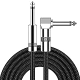
- [Low Noise High Fidelity] New bee guitar cord with 22AWG oxygen-free-copper center conductors provides enhanced signal transfer, the PVC insulation material and the high-density stranded copper double shield provide noise rejection for quiet operation
- [Ideal for Choice] New bee 1/4 straight and right angle metal connectors, ensures a secure connection in any instrument, pedal, or amp jack. L shape great fro on stage guitar stands
- [Wide Compatible] Suitable for mixer, power amplifier, microphone, effector, decoder, equalizer, electoronic organ, electric guitar, electric bass and other electronic equipments. Widely used in the installation of smart home, karaoke speaker, professional stage audio, etc
- [Easy Disassemble] Making incidental repairs quick and easy! Very nice, flexible cable
- [Dont Hesite to Order] 24 hours customer services and professional technology team are standing by
Understand the [111]-field phase sequence
A field along the cubic [111] direction gives a concrete example of how local constraints and global phases appear together. At small field, one spin on each tetrahedron is selected by the field while the remaining spins on kagome sheets continue to satisfy the two-in/two-out constraint. This produces a kagome-ice regime. Increasing the field eventually favors ice-rule-breaking configurations approaching three-in/one-out. In the field–temperature diagram, the transition line between the kagome-ice regime and the higher-field state can be first order and terminate at a critical endpoint.
To visualize this sequence, use three coordinated panels at each selected field:
- Plot magnetization and defect density against field at several temperatures, marking hysteresis if the sweep direction matters.
- Render the real-space vertices, showing the field-selected spin and the locations of three-in/one-out and one-in/three-out vertices.
- Plot the reciprocal-space structure factor to show how the correlation pattern evolves as the kagome-ice constraints weaken.
Do not draw the critical endpoint as an exact coordinate unless your finite-size and sampling analysis resolves it. A 2024 study of a ferromagnetic-Ising pyrochlore demonstrates the value of combining field–temperature mapping with bulk characterization and neutron scattering rather than relying on one simulated color map.
What’s actually slowing this PC down?
Pick the symptom - the matching free tool is one click away.
Make real-space vertex and defect maps readable
Draw spins and classify vertices
Draw every spin as an arrow or elongated island whose orientation is visible at the figure’s final publication size. For each vertex, count the in and out spins and assign one of the five charge classes: two-in/two-out, three-in/one-out, one-in/three-out, four-in/zero-out or zero-in/four-out. Most spin-ice plots focus on the first three, but retaining the extreme classes in the data prevents them from being silently merged into a generic “defect.”
Use a neutral color for ice-rule vertices, one saturated color for positive charge and a contrasting color for negative charge. Keep the same sign legend across all temperatures and fields. Overlay a small marker at the vertex center so the charge remains visible when arrows overlap.
Show strings between opposite charges
When a local spin flip creates a pair of opposite monopole-like defects, subsequent flips can form a connected chain. Draw that chain as a thin line through the flipped-spin sequence, or encode it by highlighting the changed islands relative to a reference configuration. A string is a path in the spin texture; it is not a material wire and should not be confused with a lattice edge.
Rank #4

- Digital Family Calendar: BSIMB digital calendar wall touch screen puts an end to your chaotic life. Designed for busy families, the digital calendar keeps you organised and in step with your family. Assign different colours and tasks to each family member to make family scheduling easier and more intuitive.
- Easy Setup and Auto-Sync: Plug in, connect to WLAN and auto-syn your electric calendar in minutes. Digital wall calendar compatible with Google calendar, iCloud calendar, Outlook calendar, Cozi calendar and Yahoo calendar. Add events directly on the device or through the ecalendar app. Electronic calendar stays current whether you're at work or traveling—no manual updates needed.
- All-In-One Home Assistant: Smart calendar builds habits and encourage independence with personalised chores. Display daily meal plan to reduce the daily ‘What's for dinner?’ stress. To-do lists keep track of everything you want. Turning chores into valuable achievements with stars and rewards, making life easier and more enjoyable.
- Manage Anytime Anywhere: BSIMB electronic calendar for family stay connected with the powerful ecalendar app. Access and manage your digital wall calendar anytime, anywhere with free features like stars & rewards, photo screensaver, chore charts, meals plans, to-do lists etc. Electronic planner paid features like Magic Import tailor advanced tools for users with special needs.
- Stay in Touch with Loved Ones: Share photos or videos from your phone to electronic wall calendar with app, instantly update your life moment, and keep in touch with your family, especially those who are far away; you can also surprise your smart calendar digital wall by sending him a wish card; it's also great for keeping tech-illiterate elders in touch with the youngsters.
Direct magnetic-force-microscopy images of kagome artificial spin ice established real-space vertex imaging as an experimentally grounded representation. For simulated images, reproduce the measurement limitation you intend to compare with: finite field of view, missing islands, orientation uncertainty or a chosen threshold. Do not imply that every bulk spin in a pyrochlore has been imaged individually when the experimental observable is instead thermodynamic or neutron-based.
Do these 3 things before closing this tab:
1Repair Windows errors before they cause bigger problems2Scan for outdated or missing drivers - takes under a minute3Clear out junk files and repair common Windows errorsSeparate magnetic defects from lattice defects
Artificial spin ice allows designed lattice edge dislocations and other geometric irregularities. A dislocation changes the connectivity or arrangement of the lattice; a monopole-like defect violates the local ice rule within an otherwise specified lattice. Use separate symbols, layers or panels—for example, gray dislocation lines and colored charge markers—so a reader cannot mistake one for the other. Topological-frustration experiments combining edge dislocations with kinetic Monte Carlo illustrate why this distinction matters.
Independent reader supportYour contribution helps us test, update, and keep practical guides available for everyone.Compute and interpret reciprocal-space structure factors
From snapshots to intensity maps
For each snapshot, Fourier transform the spin field or a defined magnetic-charge field on the lattice. A generic spin structure factor can be written as S(q) = (1/N) <|Σ_j s_j exp(i q·r_j)|²>, with the exact vector and polarization treatment stated for the model and measurement. Average over snapshots and independent seeds before plotting intensity in a reciprocal-space plane. State the reciprocal-lattice units, slice orientation and any masking or form-factor treatment used.
Read pinch points correctly
Pinch points are sharp, anisotropic features in the structure factor associated with the divergence-free correlations of a Coulomb phase. They are collective signatures: a real-space panel may show mostly two-in/two-out vertices while the reciprocal-space map still contains highly structured intensity. Cluster-algorithm work on nearest-neighbor spin ice demonstrates how high-resolution color maps can resolve these features.
Pinch points broaden or weaken when temperature, defects, finite size, disorder or instrumental resolution interrupts the ideal correlations. Do not call every cross-shaped bright feature a pinch point. Verify that its location and anisotropy match the expected reciprocal-space geometry, compare with a reference ice-rule ensemble, and report the resolution or binning that controls its width.
Crashes, No Sound, or Screen Glitches?
Random freezes, missing sound and display glitches usually trace back to one bad driver. Find and replace yours safely.Free scan · under a minuteWindows Errors? Fix Them Before They Spread
Repair common Windows errors and clear accumulated junk for a smoother, more stable PC - no reinstall needed.Free scan · no reinstallKeep reciprocal and real space synchronized
For a multipanel figure, label every panel with the same parameter tuple, such as T = ..., H = ..., field direction and disorder realization. If the real-space map is from one snapshot but the structure factor is averaged over a broad parameter range, say so explicitly; otherwise readers will assume they represent the same state.
Compare bulk and artificial spin ice without mixing observables
| Comparison axis | Bulk pyrochlore spin ice | Artificial spin ice |
|---|---|---|
| Geometry | Corner-sharing tetrahedra set by the crystal structure | Patterned nanomagnets on a designed periodic, aperiodic or defected lattice |
| Typical degrees of freedom | Often classical Ising moments in canonical Ho2Ti2O7 and Dy2Ti2O7; quantum variants require a different model | Shape-anisotropic islands with discrete easy-axis orientations; geometry and island disorder can be engineered |
| Direct local imaging | Individual bulk spins are generally not mapped optically; neutron scattering and thermodynamic measurements are common correlation and bulk probes | Magnetic-force microscopy can image island orientations and vertex populations directly |
| Control of frustration | Changed through field direction, temperature, pressure, exchange and anisotropy | Changed through lattice geometry, island shape, spacing, disorder, boundaries and deliberate edge dislocations |
| Useful defect view | Vertex-charge statistics inferred from configurations or scattering models | Real-space charge maps and string trajectories can be drawn directly from images or simulations |
| Dynamics | Often slow and constrained; equilibrium sampling may be difficult at low temperature | Kinetic switching and driven protocols can be central to the experiment |
The two platforms share the ice-rule language but not necessarily the same energy scales, equilibration mechanisms or accessible observables. A visually similar vertex map does not establish quantitative equivalence between a nanomagnet array and a bulk pyrochlore.
Choose the right Monte Carlo method
Single-spin Metropolis: baseline and diagnostic
Propose a local spin reversal, calculate the energy change and accept it with the Metropolis probability at the specified temperature. This method is easy to audit and useful for checking code, but it can become extremely slow when isolated flips create pairs of defects or when the system is trapped in a topological sector.
Loop and cluster updates: move within ice manifolds
Loop or cluster algorithms flip connected sets of spins so that the ice rule is preserved or defects move collectively. They are valuable when the purpose is to sample correlations and pinch points in an ice-rule manifold. Confirm that the move set remains ergodic for the boundaries, field and lattice geometry you use; a fast algorithm that never changes a conserved sector can produce a biased phase map.
Kinetic Monte Carlo: dynamics, disorder and switching
Kinetic Monte Carlo assigns transition rates and advances a physical or model time, making it appropriate when real-time switching, barriers, disorder or driven protocols matter. Its output is not automatically an equilibrium ensemble. Report the rate model, time units, initial condition and drive protocol, and do not infer equilibrium phase boundaries from a short nonstationary trajectory.
Common failure modes and repairs
- Every point looks identical: the simulation may not have equilibrated, or the color scale may be saturating. Inspect raw distributions, extend burn-in, and set limits from the full data range.
- Defect density is exactly zero at all temperatures: check the in/out projection, vertex indexing and whether your update code can create defects. A hard ice-rule constraint may also forbid them by construction.
- Opposite charges have the same color: the sign convention may have been discarded during rendering. Store signed
Qvalues and test a known three-in/one-out configuration. - Pinch points disappear when the grid is refined: inspect reciprocal-space binning, finite-size effects and the averaging window. A single noisy snapshot is insufficient for a correlation map.
- Hysteresis is interpreted as a thermodynamic transition: separate metastable kinetics from equilibrium evidence by running both sweep directions, longer holds and independent initial states.
- Artificial and bulk figures appear directly comparable in magnitude: normalize quantities carefully and state whether they are per spin, per vertex, per tetrahedron or instrument-scaled.
- Geometric dislocations are counted as monopoles: maintain separate lattice and spin-texture data structures and separate plot layers.
- Replicates disagree strongly: report the spread instead of hiding it. Investigate topological-sector trapping, insufficient decorrelation, disorder sampling and boundary effects.
Design publication-quality phase and defect figures
Use a consistent visual grammar
Reserve one color family for scalar phase-map values, a neutral color for ice-rule vertices and a fixed diverging pair for positive and negative charges. Use perceptually ordered maps rather than rainbow scales for continuous observables. Put units and field direction on every axis, and include a shared color bar whenever panels are meant to be compared.
Annotate transitions without overstating them
Use solid lines for boundaries supported by a defined criterion and dashed lines for guides to the eye or unresolved crossover regions. Mark the location of a critical endpoint only with an uncertainty region if finite-size data do not determine a single coordinate. Include representative line cuts beneath a two-dimensional map so readers can see the peak, jump or smooth evolution behind each contour.
Make dense real-space views scannable
For large lattices, provide a full-field overview and one enlarged crop containing the vertex legend, arrows and string annotation. If arrows are too small to resolve, plot the island body or a line segment with a clearly defined direction. State whether boundaries are periodic, open or cropped from a larger periodic simulation.
Quick wins for a faster PC:
Fix the driver behind crashes, sound loss and screen glitchesFind Drivers →Repair Windows errors before they cause bigger problemsFix Now →Scan for outdated or missing drivers - takes under a minuteDriver Scan →A reproducible checklist
- State the lattice, boundary conditions, Hamiltonian, local-axis convention and charge sign.
- List temperature, field magnitude, field direction and any pressure, anisotropy or disorder parameters.
- Identify the update algorithm, equilibration length, sampling interval, number of independent seeds and system size.
- Define every plotted observable, normalization and uncertainty estimator.
- Use the same parameter point for synchronized real-space and reciprocal-space panels.
- Separate geometric lattice defects from ice-rule violations in both data and graphics.
- Distinguish equilibrium averages, driven steady states and individual snapshots.
- Test finite-size effects and state whether a feature is a transition, crossover or unresolved candidate.
- Preserve raw configurations and metadata so charge histograms, strings and structure factors can be regenerated.
A phase diagram becomes scientifically useful when a reader can trace a colored pixel to a defined ensemble, a vertex marker to an explicit in/out rule and a reciprocal-space feature to the same configurations. That chain of definitions is more important than visual complexity: it prevents a local defect map, a thermodynamic boundary and a Coulomb-phase signature from being mistaken for one another.
Quick Recap
Product prices and availability are accurate as of the date/time indicated and are subject to change. Any price and availability information displayed on Amazon at the time of purchase will apply.

