How to Run Your First Quantum Circuit on a Free Cloud Simulator

The quickest free route is IBM Quantum Composer. Open it in a browser, place a Hadamard gate on one qubit, connect that qubit to a second with a controlled-NOT gate, measure both, and run the circuit on the simulator. The histogram should contain mostly 00 and 11 results. You do not need quantum hardware; a browser, notebook, or local simulator is enough.

What you are going to build

Your first circuit will be a two-qubit Bell-state circuit. IBM describes this as a circuit in which “two qubits become maximally entangled.” It is small enough to understand gate by gate, yet it demonstrates the ideas that make quantum computing different from ordinary bit manipulation: superposition, entanglement, measurement, repeated sampling, and statistical results.

#	Preview	Product	Price
1		TOZO A1 Wireless Earbuds Bluetooth 5.3 Light Weight in Ear Headphones | IPX5 Waterproof,2 Mics for...	$13.98	Buy on Amazon
2		Smart Watch for Men Women Compatible with iPhone Samsung Android Phone 1.69 inch Full Touch Screen...	$17.99	Buy on Amazon
3		New Bee Guitar Cable 10ft Electric Instrument Bass AMP Cord | 6.35mm Jack, Durable Design, Stage and...	$8.99	Buy on Amazon
4		BSIMB 15.6" Digital Family Calendar & Chore Chart, No Subscription Fees	$199.99	Buy on Amazon
5		Pokemon FireRed and LeafGreen Strategy Guidebook: Affordable & Unofficial Strategy Guide...	$19.98	Buy on Amazon

As an Amazon Associate I earn from qualifying purchases.

The circuit starts with both qubits in the state |0⟩. A Hadamard gate, written H, puts the first qubit into an equal superposition of 0 and 1. A controlled-NOT, or CNOT, flips the second qubit only when the first qubit is 1. Together, those operations create the state (|00⟩ + |11⟩) / √2. Measuring both qubits therefore produces matching values: 00 or 11. A single run is random, but many runs reveal the approximately even pattern.

A simulator calculates the circuit model in software and samples it repeatedly. It does not create a physical entangled pair, and it does not reproduce every imperfection of a real processor unless you deliberately add a noise model. That makes it ideal for learning circuit logic before you use scarce or billable hardware time.

#1 Best Overall

Sale

TOZO A1 Wireless Earbuds Bluetooth 5.3 Light Weight in Ear Headphones | IPX5 Waterproof,2 Mics for AI Calls,Immersive Premium Sound Bass Headset with Charging Case,32 EQ via App Black

• [Ultra-Lightweight Ear Buds Designed for Small Ears] Each earbud weighs only 3.7g and features a compact, ergonomic in-ear design made especially for small ears. Secure, low-profile, and comfortable for workouts, all-day wear or overnight sleeping.The ultra-slim profile sits flush in your ear with no hard edges poking or rubbing, so you can even sleep on your side without discomfort.
• [Immersive Stereo Sound with TOZO OrigX Technology] TOZO OrigX tuning delivers clear vocals, balanced mids, and natural stereo sound for music, podcasts, and videos.
• [Long Battery Life for Daily Use] Get up to 7 hours of playtime on a single charge, with up to 32 hours total using the charging case—ideal for workdays, commuting, and extended listening sessions.
• [Bluetooth 5.3 & Stable Connection] Bluetooth 5.3 provides fast pairing, stable wireless performance, and reduced dropouts as you move around home or office.
• [Deep Bass with Clear Vocals] High-performance drivers produce punchy bass while keeping vocals clean and detailed for everyday listening.

$13.98

Buy on Amazon

Run the Bell state in IBM Quantum Composer

Composer is the least complicated starting point because the circuit is assembled visually in a browser. IBM’s Composer documentation includes a guided first circuit, and IBM also documents a quickstart that builds and runs a circuit in under two minutes without a sign-in or API key. Interface labels can change, but the workflow remains the same.

1. Open IBM Quantum Composer. Start a new circuit and wait for the qubit wires and gate palette to appear.
2. Use two qubits. Keep the default two-wire layout if it is offered. The upper wire is conventionally called qubit 0 and the lower wire qubit 1.
3. Add a Hadamard gate. Place H on qubit 0 at the first time step. This creates the superposition needed for the Bell state.
4. Add a controlled-NOT. Place a CNOT with its control on qubit 0 and its target on qubit 1 at the next time step. The control and target must be in that direction; reversing them produces a different circuit.
5. Measure both qubits. Add measurement operations to qubit 0 and qubit 1. If Composer offers an automatic measurement control, use it; otherwise place one measurement on each wire.
6. Choose the simulator. Select the available simulator execution option rather than a physical quantum processor. For a first run, a few hundred or 1,000 shots is enough to see the distribution.
7. Run and inspect the histogram. Execute the circuit and open the result visualization. The two tall bars should correspond to 00 and 11; 01 and 10 should be absent or extremely rare in an ideal simulation.

If your first histogram is not exactly 50/50, that is normal. Each shot is a random sample from the Bell-state probabilities. With 100 shots, a result such as 47 instances of 00 and 53 of 11 is entirely plausible. Increasing the shot count makes the proportions tend toward one half, but it never makes an individual shot deterministic.

Understand every operation in the circuit

Initialization

Simulators normally initialize each qubit to |0⟩ unless you specify another state. In computational-basis notation, two initialized qubits are |00⟩. This is a starting condition, not a measurement result you have already observed.

Hadamard: creating a balanced choice

The Hadamard transforms |0⟩ into (|0⟩ + |1⟩) / √2. Before measurement, the qubit is described by amplitudes for both basis states. The simulator stores those amplitudes and calculates how later gates change them; it is not simply selecting a hidden classical 0 or 1.

CNOT: correlating the qubits

The CNOT leaves the target unchanged when the control is 0 and flips the target when the control is 1. Applied to the superposition created by the Hadamard, it maps the two branches to |00⟩ and |11⟩. The result is an entangled state: measuring one qubit predicts the other in the same measurement basis.

Measurement and shots

Measurement converts the quantum state into classical bit strings. A simulator run with 1,000 shots performs that sampling 1,000 times and reports counts. The counts are evidence of the probability distribution, not a list of 1,000 different quantum states that remain available after measurement.

Rank #2

Sale

Smart Watch for Men Women Compatible with iPhone Samsung Android Phone 1.69 inch Full Touch Screen IP68 Waterproof Bluetooh Fitness Tracker Heart Rate/Sleep Monitor (Black)

• 【IP68 Waterproof Multifunctinal Smart Watch】Torjalph fitness activity tracker smart watch is IP68 waterproof technology ,you can wear it when swimming,handwashing,it's rain-proof which means that you perform multiple exercise modes outside without worrying about sweat or rain corroding your fitness smart watch,and this watch equipped with a 230 mAh large capacity battery magnetic charging ,and this sports activity tracker watch can be used 5-7 days If fully charged.
• 【Larger 1.83'' Full Screen Watch & Multi-dial Selection】1.83 inch full HD color touch screen smart watch for men / women provides excellent 240*284 resolution image quality ,This Bluetooth smart watch offers a better touch experience and remarkable immersion and ,more than 200 watch faces for you to choose from App"Da Fit ", you can change the dial style according to your mood to wear keeping the world on your wrist
• 【Accurate Activity Tracker Smart Watch 】sports watch activity tracker uses sweat and dust resistant breathable silicone strap, our Fitness Tracker Smart Watch for Android iOS Phones supports 12 sports modes,walking,running,bicycle,swimming,badminton,basketball,football,rope skipping. This bluetooth calls smart watch for men women is lightweight and stylish, bringing more convenient and relaxing sports experience while also providing more protection.
• 【Your 24 Hour Personal Daily Health Monitor】Fitness watch for women men full touch screen IP67 waterproof bluetooth smartwatch for Android iOS Phones with heart rate blood pressure monitor multifunction Andriod smart watch with steps counter sleep monitor sports fitness watch, monitoring blood oxygen saturation allows you to understand your physical condition in real time to track fitness progress ,to know your health status in time.
• 【More Functions Bluetooth Call Smart Watch】This fitness activity smart watch full screen for iPhone and Android phones includes a bunch of new features including:The bluetooth smart watch can hang up the phone, receive and display WhatsAPP /Text /Facebook /Twitter /Messenger reminder.Support sedentary reminder, alarm clock, stopwatch, timer,weather information,music control, remote camera control compatible with Android 5.0 and above or iOS 9.0 and above smartphones.

$17.99

Buy on Amazon

Free usage, accounts, and changing allowances

“Free” describes a current provider allowance, not a permanent promise that every simulator or processor is unlimited. Check the provider’s live terms before running large jobs, especially when a cloud account is attached to a billing profile.

You can complete the Bell-state exercise entirely locally or in a free notebook. A cloud account becomes relevant when you want managed execution, provider-specific simulators, job history, or a route toward real hardware.

Run the same circuit with Qiskit in Google Colab

Qiskit is the best next step when you want a reproducible script instead of a drag-and-drop circuit. IBM’s “Build and run your first quantum program” lesson is designed for a fresh Google Colab runtime. The lesson installs Qiskit, the Aer simulator package, and the IBM Runtime client, then lets you choose simulation rather than a real device.

Install the packages

In a new Colab cell, install the packages used by the lesson:

!pip install qiskit qiskit-aer qiskit-ibm-runtime

Restart the runtime only if Colab asks you to do so after installation. For a local-only Bell-state run, the IBM Runtime client is not required, but it is included in the lesson so that the same notebook can later be adapted for IBM services.

Create, simulate, and count results

from qiskit import QuantumCircuit
from qiskit_aer import AerSimulator

circuit = QuantumCircuit(2, 2)
circuit.h(0)
circuit.cx(0, 1)
circuit.measure([0, 1], [0, 1])

simulator = AerSimulator()
job = simulator.run(circuit, shots=1000)
result = job.result()
print(result.get_counts())

The output is a dictionary whose keys are measured bit strings and whose values are counts. You should see 00 and 11 with totals near 1,000 combined. Qiskit’s bit-string display convention can make the left-to-right order look reversed compared with the wire diagram because classical bit 0 is commonly printed on the right. If the counts are correct but the visual order surprises you, inspect the circuit’s qubit-to-classical-bit mapping rather than changing the gates.

Rank #3

New Bee Guitar Cable 10ft Electric Instrument Bass AMP Cord | 6.35mm Jack, Durable Design, Stage and Home Studio Use, Low Noise Shielded Electric Cord for Bass, Keyboard, Amp, Mixer

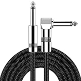
• [Low Noise High Fidelity] New bee guitar cord with 22AWG oxygen-free-copper center conductors provides enhanced signal transfer, the PVC insulation material and the high-density stranded copper double shield provide noise rejection for quiet operation
• [Ideal for Choice] New bee 1/4 straight and right angle metal connectors, ensures a secure connection in any instrument, pedal, or amp jack. L shape great fro on stage guitar stands
• [Wide Compatible] Suitable for mixer, power amplifier, microphone, effector, decoder, equalizer, electoronic organ, electric guitar, electric bass and other electronic equipments. Widely used in the installation of smart home, karaoke speaker, professional stage audio, etc
• [Easy Disassemble] Making incidental repairs quick and easy! Very nice, flexible cable
• [Dont Hesite to Order] 24 hours customer services and professional technology team are standing by

$8.99

Buy on Amazon

Make the result easier to interpret

Run the cell several times and compare the counts. The exact numbers change because the simulator samples randomly. Add a histogram in a later cell if you want a chart, but keep the raw count dictionary: it is the portable result that can be saved, tested, or compared with another simulator.

Run it with Amazon Braket

Amazon Braket gives you two distinct ways to simulate. The local simulator runs through the SDK without sending the circuit to a managed quantum device. Managed simulators run as AWS jobs and consume the applicable service allowance. AWS documents both a free local simulator and one hour of on-demand simulator time per month through the AWS Free Tier.

Use the local simulator

!pip install amazon-braket-sdk

from braket.circuits import Circuit
from braket.devices import LocalSimulator

circuit = Circuit().h(0).cnot(0, 1)
device = LocalSimulator()
result = device.run(circuit, shots=1000).result()
print(result.measurement_counts)

AWS’s Bell-state example uses the same gate sequence, Circuit().h(0).cnot(0,1). Its documented 1,000-shot example produced Counter({'11': 503, '00': 497}). Those exact counts are an illustration of sampling, not a required answer for your run.

Understand the SV1 option

AWS describes SV1 as an on-demand state-vector simulator for circuits up to 34 qubits. That capacity is a simulator specification, not a guarantee that every 34-qubit circuit will be fast or inexpensive: state-vector memory and runtime grow rapidly as qubits and operations increase. Use the local simulator for small experiments and reserve managed execution for jobs that need AWS-hosted infrastructure or a provider-specific workflow.

Protect an AWS account

Before submitting a managed job, verify the selected device, region, shot count, and current Free Tier status in the AWS console. Stop notebook runtimes and remove test resources when finished. The Free Tier allowance is monthly and conditional; do not treat it as an unlimited cloud budget.

Try Google Cirq in Colab

Cirq is a Python framework centered on circuit construction and simulation. Google’s setup tutorial uses Google Colab, which avoids a local Python installation for the first exercise.

Rank #4

BSIMB 15.6" Digital Family Calendar & Chore Chart, No Subscription Fees

• Digital Family Calendar: BSIMB digital calendar wall touch screen puts an end to your chaotic life. Designed for busy families, the digital calendar keeps you organised and in step with your family. Assign different colours and tasks to each family member to make family scheduling easier and more intuitive.
• Easy Setup and Auto-Sync: Plug in, connect to WLAN and auto-syn your electric calendar in minutes. Digital wall calendar compatible with Google calendar, iCloud calendar, Outlook calendar, Cozi calendar and Yahoo calendar. Add events directly on the device or through the ecalendar app. Electronic calendar stays current whether you're at work or traveling—no manual updates needed.
• All-In-One Home Assistant: Smart calendar builds habits and encourage independence with personalised chores. Display daily meal plan to reduce the daily ‘What's for dinner?’ stress. To-do lists keep track of everything you want. Turning chores into valuable achievements with stars and rewards, making life easier and more enjoyable.
• Manage Anytime Anywhere: BSIMB electronic calendar for family stay connected with the powerful ecalendar app. Access and manage your digital wall calendar anytime, anywhere with free features like stars & rewards, photo screensaver, chore charts, meals plans, to-do lists etc. Electronic planner paid features like Magic Import tailor advanced tools for users with special needs.
• Stay in Touch with Loved Ones: Share photos or videos from your phone to electronic wall calendar with app, instantly update your life moment, and keep in touch with your family, especially those who are far away; you can also surprise your smart calendar digital wall by sending him a wish card; it's also great for keeping tech-illiterate elders in touch with the youngsters.

$199.99

Buy on Amazon

!pip install cirq

import cirq

q0, q1 = cirq.LineQubit.range(2)
circuit = cirq.Circuit(
    cirq.H(q0),
    cirq.CNOT(q0, q1),
    cirq.measure(q0, q1, key='result')
)

simulator = cirq.Simulator()
result = simulator.run(circuit, repetitions=1000)
print(result.histogram(key='result'))

The local Cirq simulator produces the same Bell-state pattern: matching outcomes dominate. Cirq’s tutorial also explains authentication for Quantum Engine access. That authentication is a separate step from running the local simulator; do not add cloud credentials merely to execute this notebook.

Choose the right beginner path

For a first success, use Composer. For repeatable experiments, use Qiskit, Braket, or Cirq in a notebook. The underlying Bell circuit is the same; the differences are setup, APIs, account handling, and how easily you can automate experiments.

Troubleshoot the first run

The histogram contains 01 or 10

• Check that the Hadamard is on qubit 0 and the CNOT control is also qubit 0.
• Confirm that the CNOT target is qubit 1, not another wire.
• Ensure both measurements occur after the gates, not before them.
• Inspect any circuit diagram or text representation for an accidental extra gate.

A tiny nonzero count can arise from a deliberately configured noise model, but an ideal simulator with the intended two-gate circuit should produce only the correlated strings.

The counts are not exactly equal

Increase the number of shots. A finite sample rarely divides perfectly in half. Compare the ratio, not whether the two numbers match digit for digit.

The notebook cannot import a package

• Run the installation cell in the same runtime that executes the circuit.
• Read the error for the package name: Qiskit’s simulator is supplied by qiskit-aer, while Cirq and Braket have their own packages.
• Restart the notebook runtime only when the environment requests it, then rerun the installation and import cells.
• Do not mix examples from different SDK versions without checking their current API names.

A managed cloud job asks for credentials or billing

Switch to the local simulator for the first lesson. A local run avoids provider authentication and demonstrates the same circuit logic. If you continue with managed execution, verify the account’s region, permissions, current free allowance, and billing settings before submitting jobs.

The simulator is slow or runs out of memory

Reduce the qubit count, circuit depth, or shot count. State-vector simulation stores amplitudes for every computational basis state, so the memory requirement grows exponentially with the number of qubits. A two-qubit Bell state is intentionally tiny; it does not imply that a simulator can handle an arbitrary large algorithm on a free notebook.

Best Value

Pokemon FireRed and LeafGreen Strategy Guidebook: Affordable & Unofficial Strategy Guide Walkthroughs

$19.98

Buy on Amazon

Useful experiments after the Bell state

Change the measurement basis

Insert a Hadamard immediately before measuring a qubit and compare the histogram. You are no longer measuring the same observable as the original circuit, so the distribution changes even though the state-preparation gates are unchanged. This is a practical way to see that measurement basis matters.

Remove one gate at a time

Run three variants: only the Hadamard, only the CNOT applied to initialized qubits, and the complete circuit. The first shows a roughly even distribution on one qubit; the second has no effect when its control starts at 0; the complete circuit produces correlation. Keeping the shot count constant makes the comparison meaningful.

Add a third qubit carefully

Do not assume that adding a wire creates a three-qubit entangled state. Start by preparing the two-qubit Bell pair and leave the third qubit untouched, then measure all three. The third qubit should remain 0 while the first two match. This separates “more qubits” from “more entanglement.”

Compare simulators

Implement the same gate order in Composer, Qiskit, Braket, and Cirq. Record the shot count, bit-string convention, and result counts. Small differences in counts are sampling noise; systematic differences usually indicate a reversed control-target order, a different measurement mapping, or a different initial state.

When simulation is no longer enough

Simulation is the right tool for learning syntax, checking a circuit’s ideal behavior, and building intuition. A real quantum processor adds calibration drift, gate errors, readout errors, connectivity constraints, queue time, and device-specific compilation. Those effects can make 01 and 10 appear in a Bell-state histogram even when the ideal simulator never produces them.

Move to hardware only after the simulator result is understood and the circuit is saved in a reproducible form. Keep the original ideal counts as a baseline, document the device and date, and use the same shot count when comparing runs. Free access and queue availability change, so check the provider’s current terms immediately before submitting a hardware job.

Which option should you use?

Use IBM Quantum Composer if your priority is seeing a circuit and histogram with almost no setup. Use Qiskit if you want Python control and an easy path to scripted experiments. Use Amazon Braket if you already use AWS or want one SDK that distinguishes local simulation from managed devices. Use Cirq if its Python circuit model and Google-oriented workflow match your learning goals. All four can teach the same first lesson: a Hadamard followed by a CNOT creates correlated measurements, and repeated shots reveal probabilities rather than a single predetermined answer.

Quick Recap

SaleBestseller No. 1

TOZO A1 Wireless Earbuds Bluetooth 5.3 Light Weight in Ear Headphones | IPX5 Waterproof,2 Mics for AI Calls,Immersive Premium Sound Bass Headset with Charging Case,32 EQ via App Black

$13.98

SaleBestseller No. 2

Smart Watch for Men Women Compatible with iPhone Samsung Android Phone 1.69 inch Full Touch Screen IP68 Waterproof Bluetooh Fitness Tracker Heart Rate/Sleep Monitor (Black)

$17.99

Bestseller No. 3

New Bee Guitar Cable 10ft Electric Instrument Bass AMP Cord | 6.35mm Jack, Durable Design, Stage and Home Studio Use, Low Noise Shielded Electric Cord for Bass, Keyboard, Amp, Mixer

[Easy Disassemble] Making incidental repairs quick and easy! Very nice, flexible cable

$8.99

Bestseller No. 4

BSIMB 15.6" Digital Family Calendar & Chore Chart, No Subscription Fees

$199.99

Bestseller No. 5

Pokemon FireRed and LeafGreen Strategy Guidebook: Affordable & Unofficial Strategy Guide Walkthroughs

$19.98

Product prices and availability are accurate as of the date/time indicated and are subject to change. Any price and availability information displayed on Amazon at the time of purchase will apply.

Amazon Braketbeginner guideBell stateGoogle CirqIBM Quantum ComposerQiskitQuantum Computingquantum simulator