A CMB power spectrum is a map of fluctuation strength by angular scale. Read the multipole ℓ from left to right, verify whether the vertical axis is Cℓ or Dℓ = ℓ(ℓ + 1)Cℓ/(2π), then distinguish measured bandpowers from the fitted theory curve. The first acoustic peak near ℓ ≈ 200 (roughly 1–2 degrees on the sky) marks sound waves in the early photon–baryon plasma; the later peaks, polarization spectra and their covariance carry the quantitative cosmological information.
What a CMB power spectrum represents
The cosmic microwave background (CMB) is almost uniform, with a mean temperature of about 2.73 K. Tiny temperature variations—about one part in 100,000 according to the European Space Agency (ESA)—are the imprint of conditions in the young universe. A sky map contains hot and cold patches of many sizes. A power spectrum compresses that two-dimensional map into a one-dimensional description: how much fluctuation power exists at each angular scale.

As an Amazon Associate I earn from qualifying purchases.
Because the sky is a sphere, the map is expanded in spherical harmonics rather than ordinary sine waves. The multipole number ℓ labels the harmonic order. Low ℓ modes describe broad patterns spanning a large fraction of the sky; high ℓ modes describe progressively finer structure. A useful, approximate conversion is:
angular scale θ (degrees) ≈ 180° / ℓ
This is a rule of thumb, not an exact boundary for a feature. Projection effects, the width of a peak and the way an experiment bins data all matter. Nevertheless, it lets you translate a plotted horizontal position into an intuitive angular size.
#1 Best Overall

- [Ultra-Lightweight Ear Buds Designed for Small Ears] Each earbud weighs only 3.7g and features a compact, ergonomic in-ear design made especially for small ears. Secure, low-profile, and comfortable for workouts, all-day wear or overnight sleeping.The ultra-slim profile sits flush in your ear with no hard edges poking or rubbing, so you can even sleep on your side without discomfort.
- [Immersive Stereo Sound with TOZO OrigX Technology] TOZO OrigX tuning delivers clear vocals, balanced mids, and natural stereo sound for music, podcasts, and videos.
- [Long Battery Life for Daily Use] Get up to 7 hours of playtime on a single charge, with up to 32 hours total using the charging case—ideal for workdays, commuting, and extended listening sessions.
- [Bluetooth 5.3 & Stable Connection] Bluetooth 5.3 provides fast pairing, stable wireless performance, and reduced dropouts as you move around home or office.
- [Deep Bass with Clear Vocals] High-performance drivers produce punchy bass while keeping vocals clean and detailed for everyday listening.
Start by identifying both axes and the plotting convention
The horizontal axis: multipole ℓ
Read the horizontal axis as spherical-harmonic order, usually written ℓ or, in some Planck documentation, L. The U.S. Planck Data Center describes the graph as the amount of power at each multipole if the image were decomposed into spherical harmonics of order “L.” A point near ℓ = 2 represents a pattern covering very large angles; a point near ℓ = 2,000 represents structure of only a few arcminutes.
Some plots begin at ℓ = 2 because the monopole (ℓ = 0) is the mean temperature and the dipole (ℓ = 1) is dominated by our motion relative to the CMB, neither of which is normally treated as primordial anisotropy in the plotted spectrum. Check the axis limits before comparing two figures: one may show only the well-measured range while another includes the largest-scale modes.
The vertical axis: Cℓ versus Dℓ
The fundamental spectrum is Cℓ, the variance assigned to each multipole. Popular review figures often plot the rescaled quantity
Dℓ = ℓ(ℓ + 1) Cℓ / (2π)
instead. Dℓ is still the same harmonic information, but its scaling makes acoustic features easier to see: a scale-invariant spectrum appears approximately flat in Dℓ, whereas it does not look flat in Cℓ. Never compare the apparent height or slope of two plots until you know which convention each uses.
Power is usually expressed in microkelvin squared (µK2). A spectrum is a variance, so the square on the unit is essential. Temperature anisotropy itself is often discussed as a dimensionless fraction, ΔT/T, while the plotted TT power is commonly in µK2.
Separate measurements from the model curve
Most spectrum figures combine measured points with a smooth theoretical line. Points may be individual multipoles or, more commonly, binned bandpowers covering a range of ℓ. The line is generally a best-fit ΛCDM prediction, not a direct observation and not necessarily an independent forecast.
Rank #2

- 【IP68 Waterproof Multifunctinal Smart Watch】Torjalph fitness activity tracker smart watch is IP68 waterproof technology ,you can wear it when swimming,handwashing,it's rain-proof which means that you perform multiple exercise modes outside without worrying about sweat or rain corroding your fitness smart watch,and this watch equipped with a 230 mAh large capacity battery magnetic charging ,and this sports activity tracker watch can be used 5-7 days If fully charged.
- 【Larger 1.83'' Full Screen Watch & Multi-dial Selection】1.83 inch full HD color touch screen smart watch for men / women provides excellent 240*284 resolution image quality ,This Bluetooth smart watch offers a better touch experience and remarkable immersion and ,more than 200 watch faces for you to choose from App"Da Fit ", you can change the dial style according to your mood to wear keeping the world on your wrist
- 【Accurate Activity Tracker Smart Watch 】sports watch activity tracker uses sweat and dust resistant breathable silicone strap, our Fitness Tracker Smart Watch for Android iOS Phones supports 12 sports modes,walking,running,bicycle,swimming,badminton,basketball,football,rope skipping. This bluetooth calls smart watch for men women is lightweight and stylish, bringing more convenient and relaxing sports experience while also providing more protection.
- 【Your 24 Hour Personal Daily Health Monitor】Fitness watch for women men full touch screen IP67 waterproof bluetooth smartwatch for Android iOS Phones with heart rate blood pressure monitor multifunction Andriod smart watch with steps counter sleep monitor sports fitness watch, monitoring blood oxygen saturation allows you to understand your physical condition in real time to track fitness progress ,to know your health status in time.
- 【More Functions Bluetooth Call Smart Watch】This fitness activity smart watch full screen for iPhone and Android phones includes a bunch of new features including:The bluetooth smart watch can hang up the phone, receive and display WhatsAPP /Text /Facebook /Twitter /Messenger reminder.Support sedentary reminder, alarm clock, stopwatch, timer,weather information,music control, remote camera control compatible with Android 5.0 and above or iOS 9.0 and above smartphones.
ESA explains that Planck measurements are shown with error bars accounting for instrumental measurement uncertainty and an estimate of the uncertainty caused by the limited number of sky points available for the measurement. That second contribution is cosmic variance. At low ℓ, the universe provides only a small number of independent modes, so even a perfect instrument could measure a spectrum that differs from the ensemble-average theory.
What’s actually slowing this PC down?
Pick the symptom - the matching free tool is one click away.
Before judging agreement, inspect the legend and caption:
- Are the points raw, foreground-cleaned, or cross-spectra formed from independent data splits?
- Are they unbinned multipoles or bandpowers with a window function?
- Is the line fitted to these same points, to another experiment, or to a fixed reference cosmology?
- Do the error bars show only diagonal uncertainties, while correlations between bins are supplied separately in a covariance matrix?
A point that appears far from a smooth line is not automatically anomalous. Significance requires the full covariance, the model parameters that were allowed to vary and the range of multipoles included in the likelihood.
Read the spectrum from large angles to fine structure
Low ℓ: the largest angular scales
The far-left region corresponds to broad temperature patterns. Standard diagrams label a low-ℓ Sachs–Wolfe plateau, where gravitational redshifting at the surface of last scattering contributes strongly. At still lower multipoles, the integrated Sachs–Wolfe effect can produce a rise associated with evolving gravitational potentials, especially when dark energy becomes dynamically important.
These modes have the largest fractional uncertainties because only a few independent spherical-harmonic modes exist. A low-ℓ fluctuation can therefore be a statistically ordinary realization of the same cosmological model. Planck’s 2013 explanatory graphic described large-angle fluctuations between about 90° and 6° as roughly 10% weaker than its best-fit standard model; that historical statement should not be generalized into a permanent or universal anomaly.
The Tool Desk
Outbyte PC Repair FREEClear out junk files and repair common Windows errorsFree Scan →Outbyte Driver Updater FREEScan for outdated or missing drivers - takes under a minuteDriver Scan →The first acoustic peak near ℓ ≈ 200
The most recognizable landmark is the first temperature peak around ℓ = 200. The Planck Data Center associates this multipole with angular scales of roughly 1–2 degrees. Using 180°/ℓ gives about 0.9° as a simple scale estimate; the quoted 1–2° range reflects the finite width of the feature and the distinction between a harmonic scale and a spot diameter.
Rank #3
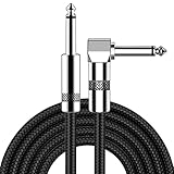
- [Low Noise High Fidelity] New bee guitar cord with 22AWG oxygen-free-copper center conductors provides enhanced signal transfer, the PVC insulation material and the high-density stranded copper double shield provide noise rejection for quiet operation
- [Ideal for Choice] New bee 1/4 straight and right angle metal connectors, ensures a secure connection in any instrument, pedal, or amp jack. L shape great fro on stage guitar stands
- [Wide Compatible] Suitable for mixer, power amplifier, microphone, effector, decoder, equalizer, electoronic organ, electric guitar, electric bass and other electronic equipments. Widely used in the installation of smart home, karaoke speaker, professional stage audio, etc
- [Easy Disassemble] Making incidental repairs quick and easy! Very nice, flexible cable
- [Dont Hesite to Order] 24 hours customer services and professional technology team are standing by
The peak is a snapshot of acoustic oscillations in the tightly coupled photon–baryon fluid before recombination. Dark-matter potential wells seeded density perturbations. Radiation pressure pushed the plasma outward while gravity pulled it back, creating sound waves. At recombination, the phase of those oscillations was projected onto the sky. Modes caught near maximum compression produce enhanced temperature power at the first peak.
Later peaks and troughs
Additional peaks and intervening troughs are higher acoustic harmonics: modes that completed different fractions of an oscillation by last scattering. Their positions measure the projected acoustic scale and therefore constrain spatial geometry when combined with the expansion history. Their relative heights encode physical effects rather than a simple repeating pattern.
Baryons add inertia to the photon fluid. This “baryon loading” changes the balance between compression and rarefaction, generally enhancing odd-numbered compression peaks relative to even-numbered ones. The total matter density, primordial fluctuation amplitude and spectral tilt also alter the sequence. Reliable parameter estimates use all peaks together, not a single height or a hand-measured ratio.
The high-ℓ damping tail
At sufficiently small scales, photon diffusion before recombination smooths fluctuations. This diffusion, often called Silk damping, produces the declining damping tail at high ℓ. The tail is sensitive to the physical conditions before recombination and to how an experiment models its beam, calibration and unresolved foreground emission.
High-ℓ points can look precise because there are many modes, but they are not automatically cleaner. Galactic dust and synchrotron radiation, extragalactic point sources and the thermal and kinetic Sunyaev–Zel’dovich effects contribute power. NASA’s LAMBDA comparative TT, TE and EE plots, for example, show spectra with foreground and Sunyaev–Zel’dovich contributions marginalized. Check whether the displayed curve has undergone the same treatment.
Why there are TT, TE and EE curves
CMB photons carry temperature information and linear polarization. The standard spectra describe auto-correlations or cross-correlations of those fields:
Rank #4

- Digital Family Calendar: BSIMB digital calendar wall touch screen puts an end to your chaotic life. Designed for busy families, the digital calendar keeps you organised and in step with your family. Assign different colours and tasks to each family member to make family scheduling easier and more intuitive.
- Easy Setup and Auto-Sync: Plug in, connect to WLAN and auto-syn your electric calendar in minutes. Digital wall calendar compatible with Google calendar, iCloud calendar, Outlook calendar, Cozi calendar and Yahoo calendar. Add events directly on the device or through the ecalendar app. Electronic calendar stays current whether you're at work or traveling—no manual updates needed.
- All-In-One Home Assistant: Smart calendar builds habits and encourage independence with personalised chores. Display daily meal plan to reduce the daily ‘What's for dinner?’ stress. To-do lists keep track of everything you want. Turning chores into valuable achievements with stars and rewards, making life easier and more enjoyable.
- Manage Anytime Anywhere: BSIMB electronic calendar for family stay connected with the powerful ecalendar app. Access and manage your digital wall calendar anytime, anywhere with free features like stars & rewards, photo screensaver, chore charts, meals plans, to-do lists etc. Electronic planner paid features like Magic Import tailor advanced tools for users with special needs.
- Stay in Touch with Loved Ones: Share photos or videos from your phone to electronic wall calendar with app, instantly update your life moment, and keep in touch with your family, especially those who are far away; you can also surprise your smart calendar digital wall by sending him a wish card; it's also great for keeping tech-illiterate elders in touch with the youngsters.
| Spectrum | Meaning | How to read it |
|---|---|---|
| TT | Temperature anisotropy correlated with itself | The familiar acoustic peak train and damping tail. |
| EE | Parity-even E-mode polarization correlated with itself | Polarization generated by velocity and quadrupole anisotropies in the photon–baryon fluid. |
| TE | Temperature–E-mode cross-correlation | Can be positive or negative, so it crosses the zero line; its sign and phase carry information about the relation between density and velocity. |
TT and EE peaks are not expected to line up perfectly. Temperature fluctuations are strongly tied to density and gravitational potential, while polarization is sourced mainly by the fluid’s velocity and the local radiation quadrupole. The resulting EE acoustic pattern is approximately out of phase with TT, as summarized by the Particle Data Group (PDG).
Free tools Windows power users keep installed
One-click scans. No signup required.
TE is not an “average” of TT and EE. It is a correlation between two different maps and can have either sign. The PDG notes that because the T and E skies are correlated, measuring TE as well as TT and EE is necessary to extract the available cosmological information. A TE curve crossing zero is therefore expected physics, not a plotting mistake.
BB, TB and EB
Data releases may also provide BB, TB and EB:
- BB is the curl-like polarization component. Lensing of E modes produces a measurable BB signal; primordial gravitational waves would add a distinctive large-scale contribution, so BB is central to searches for tensor perturbations.
- TB and EB should be consistent with null expectations in a parity-conserving cosmology. Nonzero values are useful diagnostics for polarization-angle calibration, leakage between temperature and polarization, or other systematics.
Do not infer a primordial signal from a visually elevated BB curve without checking lensing, foreground cleaning, noise bias removal and the experiment’s null tests.
What peak positions and heights tell you
The first peak’s location primarily constrains the apparent angular size of the sound horizon at recombination. That quantity depends on the physical sound horizon and the geometry that projects it onto today’s sky. Shifting the whole peak pattern horizontally can therefore indicate a change in spatial curvature or in the distance to last scattering, although parameter degeneracies mean that CMB data are normally combined with other observations.
Peak heights and ratios respond to several ingredients at once:
Quick wins for a faster PC:
Scan for outdated or missing drivers - takes under a minuteDriver Scan →Repair Windows errors before they cause bigger problemsFix Now →Fix the driver behind crashes, sound loss and screen glitchesFind Drivers →- Baryon density: changes the inertia of the photon–baryon fluid and the odd/even peak contrast.
- Total matter density: changes gravitational driving and the expansion rate around recombination.
- Primordial amplitude: sets the overall fluctuation normalization.
- Primordial tilt: changes power gradually with scale, altering the envelope of the peaks.
- Diffusion and recombination physics: shape the damping tail.
These are coupled effects. A higher peak can result from more than one parameter, and changing one parameter often shifts several features simultaneously. Cosmological analyses therefore fit the complete TT, TE and EE spectra, their beam and calibration nuisance parameters, foreground amplitudes and the full covariance matrix. Reading one peak by eye is useful for orientation, not for a precision measurement.
Independent reader supportYour contribution helps us test, update, and keep practical guides available for everyone.How to decide whether a feature is real
Cosmic variance at low multipoles
For each ℓ there are roughly 2ℓ + 1 independent m modes on a full sky. At low ℓ that number is small, so the measured power has an irreducible sample variance. Masking the Galaxy reduces the effective number of modes further and introduces correlations between neighboring multipoles. A broad low-ℓ departure within the quoted covariance is not evidence of an instrument failure or new physics.
Noise, beams and calibration at high multipoles
At high ℓ, detector noise and the finite beam become increasingly important. Beam uncertainty changes the apparent small-scale amplitude; calibration uncertainty can move an entire spectrum up or down. Experiments usually fit nuisance parameters for these effects. If a high-ℓ residual tracks the expected beam or foreground template, it should not be interpreted as a primordial feature.
Foregrounds and frequency dependence
Unlike the CMB, many foregrounds vary strongly with observing frequency. Planck’s broad frequency coverage was used to separate CMB emission from Galactic and other sources. A published spectrum may be a component-separated map, a multifrequency likelihood result or a foreground-marginalized estimate. Those products are not interchangeable. Read the caption for the mask, frequency combination, component-separation method and foreground model.
Do these 3 things before closing this tab:
1Clear out junk files and repair common Windows errors2Scan for outdated or missing drivers - takes under a minute3Repair Windows errors before they cause bigger problemsResiduals and covariance
To test a claimed feature, subtract the theory prediction from the measured bandpowers and inspect residuals with the supplied covariance matrix. Neighboring bins can be correlated, so counting how many error bars a line appears to miss is insufficient. A valid significance calculation evaluates the correlated residual vector over a stated multipole range and accounts for any parameters refitted after the feature was noticed.
A practical step-by-step method
- Read the caption first. Record the experiment, release date, sky fraction, frequency channels, mask and whether the plot is TT, TE, EE or another spectrum.
- Identify the horizontal variable. Confirm that it is ℓ (or L), note the minimum and maximum values and estimate angular scales with 180°/ℓ.
- Identify the vertical convention. Look for Cℓ or Dℓ = ℓ(ℓ + 1)Cℓ/(2π), and record the units, normally µK2.
- Separate points from lines. Determine whether points are individual multipoles or binned bandpowers and whether the line is a best fit to the same data.
- Scan the landmarks. Locate the Sachs–Wolfe/ISW low-ℓ region, the first peak near ℓ ≈ 200, subsequent acoustic harmonics and the damping tail.
- Check the physics channel. In TT, focus on temperature acoustic structure; in EE, expect a different phase; in TE, expect sign changes.
- Inspect uncertainty treatment. At low ℓ, include cosmic variance; at high ℓ, check noise, beam, calibration and foreground marginalization.
- Use the covariance for claims. Evaluate residuals against the covariance matrix rather than relying on visual separation from the line.
Comparing two CMB spectra or datasets
When figures appear to disagree, compare the properties below before comparing the curves themselves.
| Comparison item | Why it matters | Question to ask |
|---|---|---|
| Multipole coverage | Different ℓ ranges emphasize different physical effects and systematics. | Do both include the same low-ℓ and high-ℓ modes? |
| Fields measured | TT alone contains less information than a joint TT, TE and EE analysis. | Are polarization spectra included, and are they E-mode only? |
| Frequency and sky fraction | These determine foreground separation and the number of usable modes. | Were the same channels and mask used? |
| Binning and window functions | A narrow feature can be diluted or shifted by bin averaging. | Are points raw multipoles or bandpowers? |
| Covariance | Masking, beams and binning correlate errors. | Is a full covariance matrix available? |
| Foreground treatment | Dust, synchrotron, point sources and Sunyaev–Zel’dovich signals affect especially high ℓ. | Are they cleaned, fitted, or marginalized? |
| Beam and calibration model | Small-scale amplitude and slope can change with nuisance assumptions. | Were beam and calibration uncertainties propagated? |
| Theory status | A best fit can follow the plotted data, while an external prediction provides an independent test. | Was the line fitted to these points or fixed beforehand? |
Planck’s published spectra illustrate the importance of coverage: its 2018 release documentation reports TT through ℓ = 2,508, while TE, EE, EB and BB products extend to about ℓ = 1,996. Those endpoints describe that release’s products, not a universal limit for every CMB experiment.
Worked example: interpreting a typical TT plot
Suppose a figure shows Dℓ in µK2, with points from ℓ = 2 to 2,500 and a smooth ΛCDM line. Begin at the left: broad fluctuations occupy the low-ℓ Sachs–Wolfe region, where wide error bars are expected. Move to ℓ ≈ 200: the first prominent maximum indicates the projected sound horizon and the existence of acoustic oscillations. Continue rightward: alternating maxima and minima reveal higher harmonics, while their odd/even contrast reflects baryon loading and their envelope responds to matter density and primordial tilt. Beyond the final strong peaks, the declining tail reflects diffusion damping, but its exact height also depends on foreground, beam and calibration treatment.
Outdated Drivers Are Slowing You Down
One free scan finds every outdated or missing driver and matches the right update for your exact hardware.Free scan · exact hardware matchPC Slower Than It Used to Be?
A free scan shows the junk files, broken settings and background clutter dragging Windows down - then fixes them in one click.Free scan · Windows 10 & 11If the points lie systematically above the line only at the highest ℓ, inspect the foreground and beam model before proposing a change to primordial physics. If a low-ℓ group lies below the line, compare it with the cosmic-variance covariance and check whether the model was refitted. If a TE curve changes sign while TT and EE remain positive, that is normal: cross-correlation can be negative even when both auto-spectra are positive.
Common reading mistakes and fixes
- Mistake: treating ℓ as a physical distance. Fix: it is an angular harmonic index; convert approximately with 180°/ℓ and remember the projection to the last-scattering surface.
- Mistake: assuming every plot uses the same vertical quantity. Fix: verify Cℓ versus Dℓ before comparing slopes or peak heights.
- Mistake: calling the smooth line “the data.” Fix: identify whether it is a best-fit ΛCDM curve, a fixed reference model or an independent prediction.
- Mistake: interpreting error bars as purely instrumental. Fix: low-ℓ bars include cosmic variance; read the caption for the exact construction.
- Mistake: reading a TE zero crossing as a missing signal. Fix: TE is a signed cross-spectrum and naturally changes sign.
- Mistake: using one peak to estimate one parameter. Fix: parameter constraints come from joint fits to all spectra, nuisance parameters and covariance.
- Mistake: declaring a high-ℓ excess new physics. Fix: check foreground cleaning or marginalization, beam transfer functions, calibration and unresolved sources.
- Mistake: comparing unbinned and binned curves directly. Fix: account for the bin window function and correlated errors.
The essential interpretation
A CMB spectrum is best read as a sequence of angular scales and physical processes: large-angle gravitational effects at low ℓ, acoustic oscillations culminating in a first peak near ℓ ≈ 200, higher harmonics whose positions and relative heights encode geometry and matter content, and a diffusion-damped tail at high ℓ. TT, TE and EE provide complementary views of the same photon–baryon history, while BB, TB and EB add lensing and systematics information. The plot becomes quantitatively meaningful only after its convention, data treatment, foreground model and covariance are known.
Quick Recap
Product prices and availability are accurate as of the date/time indicated and are subject to change. Any price and availability information displayed on Amazon at the time of purchase will apply.

