What’s actually slowing this PC down?
Pick the symptom - the matching free tool is one click away.
Use passband-specific theoretical coefficients as informative, nonzero-width priors, then let the coefficients adjust when the light curve can identify them. The quadratic law is a practical starting point, but its coefficients change with stellar temperature, gravity, metallicity, atmosphere model, instrument throughput and fitting convention. Fixing an uncertain pair can bias the radius ratio by percent-level amounts; fitting a physically parameterized model and propagating coefficient uncertainty is safer.
What limb darkening does to a transit light curve
A star is usually brighter at the centre of its visible disk than near its edge. In a transit, the planet therefore blocks different surface brightnesses as it moves across the disk. The resulting light curve is not determined by the planet-to-star radius ratio alone: limb darkening changes the curvature between ingress, mid-transit and egress, and it is especially important when the impact parameter is high or the data resolve ingress and egress well.

As an Amazon Associate I earn from qualifying purchases.
The effect is wavelength dependent. A stellar atmosphere can look substantially different in an optical band, a near-infrared band and a narrow spectroscopic channel. Instrument throughput also matters because a broadband detector records the atmosphere intensity profile after weighting every wavelength by the telescope, filter and detector response. A coefficient pair calculated for one passband cannot be assumed to apply to another.
The geometry and the intensity profile
Transit models describe a point on the stellar disk with μ = cos(γ), where γ is the angle between the line of sight and the emergent intensity. At disk centre, μ is 1; it approaches 0 at the stellar limb. Limb-darkening coefficients describe the normalized specific intensity, I(μ)/I(1), rather than a directly measured planet property.
#1 Best Overall

- [Ultra-Lightweight Ear Buds Designed for Small Ears] Each earbud weighs only 3.7g and features a compact, ergonomic in-ear design made especially for small ears. Secure, low-profile, and comfortable for workouts, all-day wear or overnight sleeping.The ultra-slim profile sits flush in your ear with no hard edges poking or rubbing, so you can even sleep on your side without discomfort.
- [Immersive Stereo Sound with TOZO OrigX Technology] TOZO OrigX tuning delivers clear vocals, balanced mids, and natural stereo sound for music, podcasts, and videos.
- [Long Battery Life for Daily Use] Get up to 7 hours of playtime on a single charge, with up to 32 hours total using the charging case—ideal for workdays, commuting, and extended listening sessions.
- [Bluetooth 5.3 & Stable Connection] Bluetooth 5.3 provides fast pairing, stable wireless performance, and reduced dropouts as you move around home or office.
- [Deep Bass with Clear Vocals] High-performance drivers produce punchy bass while keeping vocals clean and detailed for everyday listening.
Quadratic law
The common two-coefficient model is
I(μ)/I(1) = 1 − u1(1−μ) − u2(1−μ)2.
Its compactness makes it a good default for broadband photometry. The two coefficients can nevertheless be strongly correlated with the impact parameter and radius ratio, and a numerically precise fit does not guarantee physically plausible intensity near the limb.
Square-root and higher-order laws
The square-root law is
I(μ)/I(1) = 1 − s1(1−μ) − s2(1−√μ).
A nonlinear four-parameter law is
I(μ)/I(1) = 1 − c1(1−μ0.5) − c2(1−μ) − c3(1−μ1.5) − c4(1−μ2).
These extra terms can follow atmosphere profiles more closely, particularly in infrared or wavelength-resolved data, but every additional coefficient needs information in the light curve or a defensible prior. More flexibility is not automatically more accurate when the transit is shallow, sparsely sampled or noisy.
Why the choice and treatment of coefficients changes the planet radius
The transit depth is approximately (Rp/R*)2 for a central, uniformly bright crossing, but real data are fitted over a changing stellar intensity field. If the adopted profile is too bright or too faint near the chord crossed by the planet, the optimizer can compensate by changing Rp/R*, impact parameter, baseline terms or other transit parameters.
Published simulations illustrate the scale. Espinoza and Jordán (2015) found that fixing quadratic coefficients could produce a bias of up to approximately 3% in Rp/R*; cases in which coefficients were fitted still showed biases of about 1%. Yang and collaborators (2021) reported up to 0.82% (2.5 standard deviations) bias in Rp/R* for a quadratic law under biased priors, compared with 0.32% (1.0 standard deviation) for their nonlinear-law case. These are study-specific results, not universal error bars, but they show why coefficient uncertainty belongs in the transit error budget.
Rank #2

- 【IP68 Waterproof Multifunctinal Smart Watch】Torjalph fitness activity tracker smart watch is IP68 waterproof technology ,you can wear it when swimming,handwashing,it's rain-proof which means that you perform multiple exercise modes outside without worrying about sweat or rain corroding your fitness smart watch,and this watch equipped with a 230 mAh large capacity battery magnetic charging ,and this sports activity tracker watch can be used 5-7 days If fully charged.
- 【Larger 1.83'' Full Screen Watch & Multi-dial Selection】1.83 inch full HD color touch screen smart watch for men / women provides excellent 240*284 resolution image quality ,This Bluetooth smart watch offers a better touch experience and remarkable immersion and ,more than 200 watch faces for you to choose from App"Da Fit ", you can change the dial style according to your mood to wear keeping the world on your wrist
- 【Accurate Activity Tracker Smart Watch 】sports watch activity tracker uses sweat and dust resistant breathable silicone strap, our Fitness Tracker Smart Watch for Android iOS Phones supports 12 sports modes,walking,running,bicycle,swimming,badminton,basketball,football,rope skipping. This bluetooth calls smart watch for men women is lightweight and stylish, bringing more convenient and relaxing sports experience while also providing more protection.
- 【Your 24 Hour Personal Daily Health Monitor】Fitness watch for women men full touch screen IP67 waterproof bluetooth smartwatch for Android iOS Phones with heart rate blood pressure monitor multifunction Andriod smart watch with steps counter sleep monitor sports fitness watch, monitoring blood oxygen saturation allows you to understand your physical condition in real time to track fitness progress ,to know your health status in time.
- 【More Functions Bluetooth Call Smart Watch】This fitness activity smart watch full screen for iPhone and Android phones includes a bunch of new features including:The bluetooth smart watch can hang up the phone, receive and display WhatsAPP /Text /Facebook /Twitter /Messenger reminder.Support sedentary reminder, alarm clock, stopwatch, timer,weather information,music control, remote camera control compatible with Android 5.0 and above or iOS 9.0 and above smartphones.
The bias propagates to depth, density and any atmospheric quantity that uses the measured radius. A coefficient table without its atmosphere grid, passband, stellar inputs, μ sampling and fitting method is therefore incomplete. Never quote a radius precision derived from a transit fit while omitting uncertainty in the coefficients and in the stellar parameters used to predict them.
Which limb-darkening law should you use?
| Law | Free coefficients | When it is useful | Main limitation |
|---|---|---|---|
| Quadratic | 2 (u1, u2) |
Compact broadband model; usually the first model to try | Can miss detailed atmosphere curvature and is sensitive to biased or fixed priors |
| Square-root | 2 (s1, s2) |
Alternative two-term shape when the square-root dependence follows the observed profile better | Still constrained by only two terms; coefficients are not interchangeable with quadratic values |
| Nonlinear four-parameter | 4 (c1 through c4) |
Infrared, spectroscopic or very high signal-to-noise data; atmosphere profiles with detailed curvature | More degeneracy and computational cost; free coefficients may be unidentifiable in ordinary light curves |
Compare candidate laws on five axes: how closely they reproduce the atmosphere intensity over the μ range actually sampled by the transit; how many coefficients the data can identify; sensitivity to atmosphere and throughput mismatch; the resulting change in Rp/R* and depth; and posterior stability and computational cost. A four-coefficient fit that has smaller profile residuals but broad, highly correlated posteriors is not necessarily a better measurement than a well-constrained quadratic model.
Recommended Free Tools
A defensible workflow from stellar inputs to a transit posterior
1. Fix the stellar solution and the actual passband
Record the adopted effective temperature, surface gravity, metallicity and their uncertainties. Obtain the instrument response, including filter, optics and detector throughput, for the observation being analysed. TESS, Kepler, HST and JWST observations each require their own response curve; even two modes on the same observatory can differ.
Atmosphere coefficients are passband-specific. Updating the stellar solution without updating the coefficients creates an internally inconsistent model. Keep the throughput version and stellar-parameter source in the analysis metadata so the calculation can be reproduced.
2. Select a law appropriate to the information content
Start with the quadratic law for a compact broadband analysis. Move to a square-root, power-2 or four-parameter law when an atmosphere profile or structured residuals indicate that two quadratic terms are inadequate, especially for infrared or wavelength-resolved data. Do not select the four-parameter law solely because it has a lower training residual: the transit may not contain enough independent information to estimate four coefficients.
Rank #3
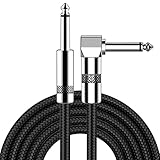
- [Low Noise High Fidelity] New bee guitar cord with 22AWG oxygen-free-copper center conductors provides enhanced signal transfer, the PVC insulation material and the high-density stranded copper double shield provide noise rejection for quiet operation
- [Ideal for Choice] New bee 1/4 straight and right angle metal connectors, ensures a secure connection in any instrument, pedal, or amp jack. L shape great fro on stage guitar stands
- [Wide Compatible] Suitable for mixer, power amplifier, microphone, effector, decoder, equalizer, electoronic organ, electric guitar, electric bass and other electronic equipments. Widely used in the installation of smart home, karaoke speaker, professional stage audio, etc
- [Easy Disassemble] Making incidental repairs quick and easy! Very nice, flexible cable
- [Dont Hesite to Order] 24 hours customer services and professional technology team are standing by
3. Generate coefficients for that star and passband
Use the chosen stellar-atmosphere grid to obtain specific intensity as a function of μ at the adopted temperature, gravity and metallicity. Integrate the intensity over the instrument response, then fit the selected analytic law to the integrated profile. Document the μ points, weights, limb-point treatment and fitting objective. Different sampling and weighting conventions produce different coefficient values even when they use the same atmosphere grid.
The Tool Desk
Outbyte PC Repair FREEClear out junk files and repair common Windows errorsFree Scan →Outbyte Driver Updater FREEFix the driver behind crashes, sound loss and screen glitchesFind Drivers →For a broadband observation, fit the throughput-weighted profile rather than copying a coefficient from a nearby filter. For a spectroscopic channel, use the channel response and wavelength-dependent atmosphere calculation. Interpolate in stellar parameters only within the documented grid range and carry interpolation or grid uncertainty into the prior width.
4. Sample quadratic coefficients with a physical parameterization
Kipping’s variables provide a practical way to sample the quadratic law. Define
q1 = (u1 + u2)2 and q2 = u1 / [2(u1 + u2)], with q1 and q2 sampled in the interval (0, 1). Recover the conventional coefficients using
u1 = 2√q1 q2u2 = √q1 (1 − 2q2).
This transformation reduces the strong correlation commonly seen when sampling u1 and u2 directly and avoids many draws that correspond to unphysical intensity profiles. Store both the sampled variables and the recovered coefficients so posterior summaries remain interpretable. The same principle applies to other laws: choose a parameterization that enforces the physical constraints of the selected profile instead of relying on a wide unconstrained box.
Rank #4

- Digital Family Calendar: BSIMB digital calendar wall touch screen puts an end to your chaotic life. Designed for busy families, the digital calendar keeps you organised and in step with your family. Assign different colours and tasks to each family member to make family scheduling easier and more intuitive.
- Easy Setup and Auto-Sync: Plug in, connect to WLAN and auto-syn your electric calendar in minutes. Digital wall calendar compatible with Google calendar, iCloud calendar, Outlook calendar, Cozi calendar and Yahoo calendar. Add events directly on the device or through the ecalendar app. Electronic calendar stays current whether you're at work or traveling—no manual updates needed.
- All-In-One Home Assistant: Smart calendar builds habits and encourage independence with personalised chores. Display daily meal plan to reduce the daily ‘What's for dinner?’ stress. To-do lists keep track of everything you want. Turning chores into valuable achievements with stars and rewards, making life easier and more enjoyable.
- Manage Anytime Anywhere: BSIMB electronic calendar for family stay connected with the powerful ecalendar app. Access and manage your digital wall calendar anytime, anywhere with free features like stars & rewards, photo screensaver, chore charts, meals plans, to-do lists etc. Electronic planner paid features like Magic Import tailor advanced tools for users with special needs.
- Stay in Touch with Loved Ones: Share photos or videos from your phone to electronic wall calendar with app, instantly update your life moment, and keep in touch with your family, especially those who are far away; you can also surprise your smart calendar digital wall by sending him a wish card; it's also great for keeping tech-illiterate elders in touch with the youngsters.
5. Use informative priors, not silently fixed numbers
Atmosphere predictions are useful as informative priors, with widths that include uncertainty in stellar parameters, model atmosphere assumptions, passband throughput and the coefficient-fitting convention. A prior with zero width treats the prediction as exact and prevents the data from correcting a mismatch. Conversely, a completely flat prior on several coefficients can make a noisy transit absorb baseline or geometric errors.
For sparse or low signal-to-noise data, informative nonzero-width priors usually provide the best bias-variance compromise. For a high signal-to-noise, well-sampled light curve, allow the coefficients to adjust or fit them jointly with the transit. Southworth and colleagues concluded in 2015 that “the best strategy to minimize the bias introduced in the transit parameters is to let them float in the transit fitting procedure.” Letting them float does not mean discarding atmosphere information; it means expressing that information as a prior rather than an irreversible constraint.
6. Fit transit and nuisance terms together
Pass the selected law and coefficients into a Mandel–Agol or equivalent analytic transit model. Integrate the model over the exposure time; evaluating it only at the exposure midpoint can distort ingress and egress when exposures are long relative to transit features. Fit baseline or detector-systematics terms simultaneously, using a correlated-noise model appropriate to the instrument.
Inspect posterior covariance among limb-darkening coefficients, impact parameter, radius ratio and baseline terms. A narrow marginal radius posterior can be misleading if it is produced by a strong, unexamined prior or by covariance with an under-modeled trend. For multiple visits or passbands, share only the parameters that are physically shared and give each band its own coefficients.
Windows Errors? Fix Them Before They Spread
Repair common Windows errors and clear accumulated junk for a smoother, more stable PC - no reinstall needed.Free scan · no reinstallCrashes, No Sound, or Screen Glitches?
Random freezes, missing sound and display glitches usually trace back to one bad driver. Find and replace yours safely.Free scan · under a minute7. Validate the profile and the inferred radius
Check residuals around ingress and egress, where an incorrect intensity profile is easiest to see. Compare posterior-predictive light curves with the observed curvature, and refit with a plausible alternate law. Examine whether the radius ratio and depth remain stable within their stated uncertainties. If the alternate law changes the radius materially, report that model dependence instead of hiding it in a single formal error bar.
8. Recompute after any stellar or instrument update
If effective temperature, gravity, metallicity, stellar-model grid or throughput calibration changes, regenerate the coefficients and refit the transit before remeasuring the planet size. NASA Exoplanet Archive guidance states that when new stellar parameters are adopted, the most-correct approach is to refit the transit with new limb-darkening coefficients in order to remeasure planet size.
Independent reader supportYour contribution helps us test, update, and keep practical guides available for everyone.How to obtain coefficients for TESS, Kepler, HST and JWST
No single coefficient table is valid for all four observatories. The procedure is the same, but the response function and often the relevant wavelength range differ.
| Observation | Required passband input | Recommended treatment |
|---|---|---|
| TESS | The TESS bandpass and the detector-throughput version used for the analysis | Generate a throughput-integrated profile for the target star; use a quadratic prior unless the light curve supports a more flexible law |
| Kepler | The Kepler response curve and the adopted stellar solution | Do not substitute TESS or generic optical coefficients; refit if the stellar inputs change |
| HST | The exact instrument and filter/grism throughput | Use the response for that mode and visit; wavelength-resolved data may justify a higher-order law |
| JWST | The exact instrument, filter or spectroscopic-channel response | Infrared profiles can require square-root, power-2 or nonlinear treatment; test residuals and posterior stability |
The table gives workflow guidance, not universal coefficient values. A published number is portable only when its atmosphere grid, stellar parameters, response curve, μ sampling and fitting method match your observation. Otherwise regenerate it or widen the prior to represent the mismatch.
Common failure modes and their fixes
| Symptom | Likely cause | Fix |
|---|---|---|
| Radius ratio changes noticeably when coefficients are fixed versus free | The light curve contains information about the profile, or the fixed prediction is biased | Use atmosphere-informed priors with nonzero width; compare posterior-predictive fits |
| Quadratic coefficients take extreme or unphysical values | Direct sampling permits invalid profiles or the data are too weak | Sample q1, q2 in (0, 1), or impose an equivalent physical parameterization |
| Different software packages return different coefficient pairs | They used different atmosphere grids, passbands, μ points or weighting rules | Record and match every convention before comparing numbers |
| Ingress and egress residuals remain structured | Law mismatch, exposure-time smearing or an unmodeled systematic | Integrate over exposure time, test an alternate law and revisit the systematics model |
| Four-parameter posteriors are broad and highly correlated | The data cannot identify four independent shape terms | Use informative priors or return to a quadratic model and report model dependence |
| A revised stellar catalogue leaves the old planet radius unchanged | Coefficients and transit were not refitted after the stellar update | Regenerate coefficients and rerun the transit inference |
What to record so the result can be reproduced
- Transit-law name and coefficient convention.
- Atmosphere grid, version, interpolation procedure and intensity sampling.
- Instrument, filter or spectroscopic channel and throughput version.
- Effective temperature, surface gravity, metallicity and uncertainties used for the star.
- Coefficient-fitting weights and treatment of the μ near the stellar limb.
- Prior centre and width for every coefficient, or the reason a coefficient was allowed to be effectively unconstrained.
- Sampling parameterization, including the transformation between
q1,q2andu1,u2. - Exposure-time integration method, baseline terms and correlated-noise treatment.
- Alternate-law checks and the resulting change in
Rp/R*, depth and other reported parameters.
Practical decision guide
- Broadband, modest signal-to-noise: generate quadratic coefficients for the exact passband and stellar solution, assign informative nonzero-width priors, sample with
q1andq2, and test whether freeing them changes the radius. - High signal-to-noise broadband transit: start with the quadratic model, then fit coefficients jointly and compare a physically plausible alternate law. Treat a law-dependent radius as a systematic uncertainty.
- Infrared or spectroscopic data: inspect the atmosphere profile and residuals; consider square-root, power-2 or nonlinear laws when the data support the extra terms.
- Sparse or noisy data: avoid fully free multi-coefficient fits. Use atmosphere predictions as priors, include their uncertainty and focus on validating radius stability.
- Updated stellar parameters or throughput: regenerate coefficients and refit before publishing a revised planet size.
Bottom line for a transit analysis
Limb darkening is part of the measurement model, not a cosmetic correction. Compute coefficients from the actual stellar atmosphere and instrument response, document how they were fitted, sample them with a physically valid parameterization, and propagate their uncertainty into the planet radius. The quadratic law is often efficient, but its coefficients are not universal; allowing appropriately informed adjustment and checking an alternate law is the reliable way to prevent the stellar intensity profile from masquerading as a change in planet size.
Quick Recap
Product prices and availability are accurate as of the date/time indicated and are subject to change. Any price and availability information displayed on Amazon at the time of purchase will apply.

