Quick wins for a faster PC:
Fix the driver behind crashes, sound loss and screen glitchesFind Drivers →Clear out junk files and repair common Windows errorsFree Scan →Scan for outdated or missing drivers - takes under a minuteDriver Scan →You can find a transit-like signal in public TESS data with a repeatable workflow: retrieve every sector for a target from MAST, inspect the untouched FITS light curve, clean and detrend it without erasing transits, search for repeating dips with Box Least Squares (BLS), then test the signal against instrumental, stellar and background-source explanations. That process produces a candidate—not automatically a planet. Validation products, catalog checks and often follow-up observations are needed before the object can be called validated or confirmed.
This guide assumes basic Python and astronomy knowledge. NASA’s instructional route uses Lightkurve with Matplotlib, NumPy and Astropy’s BLS implementation. Software interfaces change, so treat code examples as a transparent starting point and check the current package documentation before running them.

As an Amazon Associate I earn from qualifying purchases.
What counts as “finding” an exoplanet in TESS data?
A periodic dip in brightness is evidence that something is crossing, eclipsing or otherwise changing the light from a star. It is not, by itself, evidence that a planet caused it. The safest workflow uses deliberately narrow language as the evidence improves.
| Term | Meaning in a TESS analysis | What it does not establish |
|---|---|---|
| Transit-like signal | A dip or series of dips in a processed light curve that resembles a transit. | That the signal is astrophysical, periodic over the full baseline or planetary. |
| Threshold-crossing event (TCE) | A detection produced by an automated search after it passes a statistical threshold. | That the event survived human vetting or comes from the target star. |
| TESS Object of Interest (TOI) | A cataloged target selected for further review and follow-up. | That it is a confirmed planet; dispositions can change as new checks arrive. |
| Planet candidate | A signal that remains plausible after initial light-curve and contamination checks. | That false-positive scenarios have been ruled out. |
| Statistically validated planet | A candidate for which a formal analysis makes non-planet explanations sufficiently unlikely under stated assumptions. | A dynamical confirmation or a permanently settled catalog status. |
| Confirmed planet | An object whose planetary nature has been established with the evidence and follow-up appropriate to the case. | That every measured property, such as radius or mass, is equally precise. |
Report the earliest defensible status. For example, write “a transit-like signal at a period of …” while you are still testing it, rather than “we discovered a planet.”
#1 Best Overall

- [Ultra-Lightweight Ear Buds Designed for Small Ears] Each earbud weighs only 3.7g and features a compact, ergonomic in-ear design made especially for small ears. Secure, low-profile, and comfortable for workouts, all-day wear or overnight sleeping.The ultra-slim profile sits flush in your ear with no hard edges poking or rubbing, so you can even sleep on your side without discomfort.
- [Immersive Stereo Sound with TOZO OrigX Technology] TOZO OrigX tuning delivers clear vocals, balanced mids, and natural stereo sound for music, podcasts, and videos.
- [Long Battery Life for Daily Use] Get up to 7 hours of playtime on a single charge, with up to 32 hours total using the charging case—ideal for workdays, commuting, and extended listening sessions.
- [Bluetooth 5.3 & Stable Connection] Bluetooth 5.3 provides fast pairing, stable wireless performance, and reduced dropouts as you move around home or office.
- [Deep Bass with Clear Vocals] High-performance drivers produce punchy bass while keeping vocals clean and detailed for everyday listening.
Data and software you need
MAST is the starting point
The Mikulski Archive for Space Telescopes (MAST) is NASA’s official primary science archive for processed TESS data and metadata. You can search its web portal or use its programmatic services through an API or astroquery. Search by a TIC identifier, another supported name or coordinates, and record the sectors, file types and processing labels returned.
A target observed in several sectors normally has separate sector-specific light-curve files. Do not assume that one file contains the complete observing baseline. Longer coverage can reveal more transits, but it also introduces sector boundaries, gaps and changes in systematics that must be inspected.
Light curves, target pixels and validation products
TESS light-curve files are FITS time series produced from photometric extraction and systematics correction. They provide time, flux and uncertainty measurements suitable for plotting and period searches. Target Pixel Files (TPFs) preserve the pixels around the target. They let you examine the chosen aperture, nearby stars, background light and whether the apparent event is centered on the target.
MAST also distributes Data Validation (DV) products when they are available. These reports and time series contain pipeline diagnostics that are valuable during vetting; they are not a substitute for looking at the underlying pixels and light curve.
Install and version awareness
NASA’s beginner material uses Lightkurve, Matplotlib and NumPy and assumes basic Python and astronomy knowledge. The tutorial search result identifies Lightkurve 2.0.1, but that is not a guarantee that it is the current release. Follow the project’s current installation instructions and record the package versions used for a reproducible analysis. API names and defaults can change.
Rank #2

- 【IP68 Waterproof Multifunctinal Smart Watch】Torjalph fitness activity tracker smart watch is IP68 waterproof technology ,you can wear it when swimming,handwashing,it's rain-proof which means that you perform multiple exercise modes outside without worrying about sweat or rain corroding your fitness smart watch,and this watch equipped with a 230 mAh large capacity battery magnetic charging ,and this sports activity tracker watch can be used 5-7 days If fully charged.
- 【Larger 1.83'' Full Screen Watch & Multi-dial Selection】1.83 inch full HD color touch screen smart watch for men / women provides excellent 240*284 resolution image quality ,This Bluetooth smart watch offers a better touch experience and remarkable immersion and ,more than 200 watch faces for you to choose from App"Da Fit ", you can change the dial style according to your mood to wear keeping the world on your wrist
- 【Accurate Activity Tracker Smart Watch 】sports watch activity tracker uses sweat and dust resistant breathable silicone strap, our Fitness Tracker Smart Watch for Android iOS Phones supports 12 sports modes,walking,running,bicycle,swimming,badminton,basketball,football,rope skipping. This bluetooth calls smart watch for men women is lightweight and stylish, bringing more convenient and relaxing sports experience while also providing more protection.
- 【Your 24 Hour Personal Daily Health Monitor】Fitness watch for women men full touch screen IP67 waterproof bluetooth smartwatch for Android iOS Phones with heart rate blood pressure monitor multifunction Andriod smart watch with steps counter sleep monitor sports fitness watch, monitoring blood oxygen saturation allows you to understand your physical condition in real time to track fitness progress ,to know your health status in time.
- 【More Functions Bluetooth Call Smart Watch】This fitness activity smart watch full screen for iPhone and Android phones includes a bunch of new features including:The bluetooth smart watch can hang up the phone, receive and display WhatsAPP /Text /Facebook /Twitter /Messenger reminder.Support sedentary reminder, alarm clock, stopwatch, timer,weather information,music control, remote camera control compatible with Android 5.0 and above or iOS 9.0 and above smartphones.
Step 1: Choose a target and retrieve every observation
- Define the target precisely. Prefer a TIC identifier when one is available. A common name can resolve to more than one catalog entry, so verify coordinates and the intended star.
- Search MAST. Use the portal, the MAST API or
astroqueryto list TESS observations. Keep the returned table with your analysis so another reader can see which sectors and products you used. - Download all relevant sectors. A multi-sector target may return one light-curve file per sector. Download them separately before deciding whether to combine them.
- Record product choices. Note whether each file is a pipeline light curve or a TPF, whether the flux is SAP or PDC-corrected, the sector number and any quality or processing flags.
A minimal Lightkurve-style starting point is:
import lightkurve as lk

search = lk.search_lightcurve("TIC 000000000", mission="TESS")
print(search)
collection = search.download_all()
Replace the example identifier with the target you actually intend to study. Inspect the search table before downloading: duplicate products, missing sectors and different processing versions can otherwise be mixed unintentionally.
Step 2: Understand the flux before changing it
SAP and PDC-corrected flux answer different needs
SAP (simple aperture photometry) is closer to the aperture measurement made by the pipeline. PDC-corrected flux has undergone pipeline systematics correction intended to remove common instrumental trends. Neither label guarantees that a transit is preserved perfectly in every circumstance. When a feature is important, examine both where both are available and document which one drives the search.
The Tool Desk
Outbyte Driver Updater FREEScan for outdated or missing drivers - takes under a minuteDriver Scan →Outbyte PC Repair FREERepair Windows errors before they cause bigger problemsFix Now →Pipeline light curve or custom extraction?
Pipeline light curves are convenient and make a fast, reproducible first pass. A custom extraction from a TPF gives you control over the aperture and lets you test whether a nearby source or background variation is responsible. The extra control costs time and introduces choices about aperture shape, background estimation and detrending. Use the pipeline product for orientation, then move to pixels when the signal is faint, crowded or suspicious.
Step 3: Inspect the untouched time series
Plot the downloaded data before removing NaNs, clipping outliers or flattening trends. The unmodified view is your reference for detecting processing artifacts.
- Check that timestamps are sensible and identify gaps, sector boundaries and long interruptions.
- Plot flux and its uncertainty together. A dip coincident with a sudden uncertainty increase deserves caution.
- Count missing values and inspect the quality flags supplied in the FITS table.
- Look for ramps, jumps, scattered-light patterns, discontinuities or groups of points that differ from the rest of the sector.
- Keep a copy of the original light curve and write down every transformation applied later.
Lightkurve supplies methods for removing NaNs and outliers, folding data and flattening long-term trends. Those methods are operations to inspect, not automatic proof that the remaining variations are astrophysical.
Rank #3
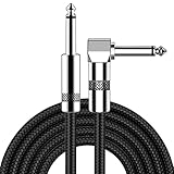
- [Low Noise High Fidelity] New bee guitar cord with 22AWG oxygen-free-copper center conductors provides enhanced signal transfer, the PVC insulation material and the high-density stranded copper double shield provide noise rejection for quiet operation
- [Ideal for Choice] New bee 1/4 straight and right angle metal connectors, ensures a secure connection in any instrument, pedal, or amp jack. L shape great fro on stage guitar stands
- [Wide Compatible] Suitable for mixer, power amplifier, microphone, effector, decoder, equalizer, electoronic organ, electric guitar, electric bass and other electronic equipments. Widely used in the installation of smart home, karaoke speaker, professional stage audio, etc
- [Easy Disassemble] Making incidental repairs quick and easy! Very nice, flexible cable
- [Dont Hesite to Order] 24 hours customer services and professional technology team are standing by
Step 4: Clean and detrend without erasing a transit
Remove unusable points transparently
Removing NaNs is usually necessary for plotting and periodograms. Outlier removal should be conservative: a single extreme point may be a cosmic-ray-like artifact, but clipping a real ingress or egress can change the measured depth and duration. Save the rejected-point mask and state the rule used.
PC Slower Than It Used to Be?
A free scan shows the junk files, broken settings and background clutter dragging Windows down - then fixes them in one click.Free scan · Windows 10 & 11Outdated Drivers Are Slowing You Down
One free scan finds every outdated or missing driver and matches the right update for your exact hardware.Free scan · exact hardware matchChoose a trend model on the transit timescale
TESS data can contain instrumental systematics and scattered light. Lightkurve correctors and pixel-level approaches can reduce those effects, but a correction model can also distort a transit when its timescale is too short or when the transit is not masked. Select a window or model that follows variability substantially longer than the expected event, compare several reasonable settings, and inspect the result against the original series.
Pixel-level decorrelation (PLD) can account for changes in the distribution of light across pixels, but its own documentation describes caveats and possible biases. Treat PLD or any cotrending method as a model with assumptions, not as a neutral filter.
A transparent workflow keeps both versions:
raw = lc.copy()
clean = lc.remove_nans().remove_outliers()
# Choose flattening settings only after estimating the likely transit duration.
flat = clean.flatten(window_length=101)
The number in this example is not universal. Change it to suit the target and test whether the candidate depth, duration and shape remain stable. If flattening creates a dip or removes one, stop and revisit the model rather than selecting the most attractive curve.
Step 5: Search for repeating events with BLS
Box Least Squares is a useful first search because a planetary transit is approximately a box-shaped decrease in flux repeated at a regular period. Lightkurve’s exoplanet tutorial uses Astropy’s BLS implementation and demonstrates stitching light curves, flattening trends and removing outliers.
Recommended Free Tools
Rank #4

- Digital Family Calendar: BSIMB digital calendar wall touch screen puts an end to your chaotic life. Designed for busy families, the digital calendar keeps you organised and in step with your family. Assign different colours and tasks to each family member to make family scheduling easier and more intuitive.
- Easy Setup and Auto-Sync: Plug in, connect to WLAN and auto-syn your electric calendar in minutes. Digital wall calendar compatible with Google calendar, iCloud calendar, Outlook calendar, Cozi calendar and Yahoo calendar. Add events directly on the device or through the ecalendar app. Electronic calendar stays current whether you're at work or traveling—no manual updates needed.
- All-In-One Home Assistant: Smart calendar builds habits and encourage independence with personalised chores. Display daily meal plan to reduce the daily ‘What's for dinner?’ stress. To-do lists keep track of everything you want. Turning chores into valuable achievements with stars and rewards, making life easier and more enjoyable.
- Manage Anytime Anywhere: BSIMB electronic calendar for family stay connected with the powerful ecalendar app. Access and manage your digital wall calendar anytime, anywhere with free features like stars & rewards, photo screensaver, chore charts, meals plans, to-do lists etc. Electronic planner paid features like Magic Import tailor advanced tools for users with special needs.
- Stay in Touch with Loved Ones: Share photos or videos from your phone to electronic wall calendar with app, instantly update your life moment, and keep in touch with your family, especially those who are far away; you can also surprise your smart calendar digital wall by sending him a wish card; it's also great for keeping tech-illiterate elders in touch with the youngsters.
For a multi-sector target, you can stitch compatible cleaned light curves after inspecting each sector:
stitched = collection.stitch()
clean = stitched.remove_nans().remove_outliers()
flat = clean.flatten(window_length=101)
Then run a BLS search over a period range and duration grid appropriate to the star and the available baseline. A schematic Lightkurve call looks like this:
import numpy as np

period_grid = np.linspace(0.5, 20.0, 10000)
duration_grid = np.array([0.05, 0.10, 0.20, 0.30])
bls = flat.to_periodogram(
    method="bls",
    period=period_grid,
    duration=duration_grid
)
best_period = bls.period_at_max_power
The ranges above are illustrative rather than a universal search prescription. A short-period grid will miss longer events; an unsuitable duration grid can weaken the peak. Record the grid, the detrending choices and the software version. The highest BLS peak is a hypothesis, not a verdict.
Fold and inspect the proposed period
Fold the light curve on the strongest period and inspect individual events, not just the phase-binned average. A credible candidate should show repeated decreases at the same phase, with broadly consistent depth and duration. Compare the folded view with each sector separately: a signal present in only one problematic segment may be an artifact, while a real event can appear at different apparent depths if systematics or dilution change.
Test nearby periods as well. Eclipsing binaries can produce a strong peak at half the orbital period, and a harmonic can look more significant than the physical period. Odd/even comparisons are therefore part of vetting, not an optional cosmetic plot.
Independent reader supportYour contribution helps us test, update, and keep practical guides available for everyone.Step 6: Vet the signal as a candidate
Test repeatability and shape
- Check that the event repeats after the proposed period across independent sectors or observing segments.
- Inspect ingress, minimum light and egress. A sharply V-shaped event, strongly changing duration or implausible baseline behavior can indicate an eclipsing binary or a poor detrending model.
- Compare odd and even events. Different depths or shapes are a warning for a binary interpretation or an incorrect period.
- Search for a secondary eclipse or other phase-dependent variation. Its presence does not by itself identify the cause, but it changes the false-positive assessment.
- Check whether the period aligns with a gap, data-quality interval, scattered-light pattern or repeated spacecraft artifact.
Check the source on the detector
A blended aperture can contain several stars. A transit-like dip may originate from a nearby eclipsing binary rather than the named target. Open the TPF, display the aperture and surrounding pixels, and compare the in-transit and out-of-transit images. Examine centroid or pixel-level motion where the product and tools support it. A shift toward a neighboring source is evidence against assigning the event automatically to the target.
Catalog crowding information is useful context, but it cannot replace the pixel check. The source of the signal must be consistent with the target position under the available spatial resolution.
Use SPOC Data Validation products
When available, inspect the pipeline’s DV reports and time series for the target. They can provide independent views of the transit model, odd/even tests, secondary-event searches and other diagnostics. Treat their conclusions as inputs to your reasoning and verify that the event is present in the underlying light curve and pixels.
Free tools Windows power users keep installed
One-click scans. No signup required.
Check the current TOI record
The TESS Science Office reviews threshold-crossing events and supplies TOI dispositions and vetting information to MAST on a nominal four-month schedule. That cadence means a catalog entry is not immutable. Check the current record and its date, and report whether the object is listed as a candidate, a false positive, or another disposition at the time you write.
Validation is a separate claim from detection
A statistical search answers, “Is there a periodic pattern that resembles a transit?” Validation asks, “After considering the data and plausible alternatives, is a planet interpretation sufficiently more likely than false-positive explanations?” The second question requires diagnostics beyond the BLS power.
Ground-based follow-up is used to distinguish true exoplanets from false positives. NASA describes a process in which candidates receive follow-up observations to determine whether they are genuine exoplanets rather than false positives. Until that evidence or a documented statistical validation supports the conclusion, call your result a candidate signal or TOI, not a confirmed planet.
Choosing an analysis path
| Choice | Best for | Trade-off to document |
|---|---|---|
| SPOC pipeline light curve | A fast, standardized first search. | Less control over aperture and systematics modeling. |
| Custom extraction from a TPF | Crowded fields, ambiguous centroids or testing alternate apertures. | More analyst choices and more ways for extraction or detrending to bias the result. |
| SAP flux | Reviewing the pipeline aperture measurement with relatively direct access to its behavior. | Instrumental trends and scattered light can remain. |
| PDC-corrected flux | A pipeline-corrected series for a convenient search. | Systematics correction is a model; inspect whether it changes the event. |
| One sector | Simple inspection and fewer discontinuities. | Shorter baseline and possibly too few transits. |
| Stitched multi-sector data | More repeated events and longer temporal coverage. | Sector offsets, gaps and changing systematics must be modeled or inspected. |
| Simple flattening | Quick removal of slow trends for exploratory work. | A poorly chosen window can attenuate, reshape or create a transit. |
| Cotrending or pixel-level correction | Explicit treatment of instrumental or pixel-distribution effects. | Model assumptions and PLD caveats can introduce bias. |
| BLS search | Locating periodic, approximately box-shaped dips. | It does not distinguish planets from binaries, background sources or artifacts. |
| Validation analysis | Testing planet and false-positive hypotheses with diagnostics and independent information. | It is slower and cannot be replaced by a periodogram peak. |
Common failure modes and recovery steps
| Symptom | Likely issue | Recovery |
|---|---|---|
| Only one dramatic dip | Noise, a data gap or a single instrumental event. | Inspect raw data and quality flags; search other sectors before assigning a period. |
| Signal appears after flattening but not before | The trend model may have created an edge or residual. | Change the flattening window, mask possible transits and compare with SAP or PDC flux. |
| Signal disappears with a different correction | The event may be entangled with systematics. | Retain both reductions, inspect pixels and treat the event as unvalidated. |
| Odd and even transits differ | Half-period binary, blended eclipsing system or incorrect period. | Test the doubled period and inspect the TPF and DV diagnostics. |
| Transit is deeper in one sector | Sector-dependent systematics, dilution changes or a background source. | Analyze sectors separately, inspect apertures and compare centroid behavior. |
| Centroid shifts during the event | The varying source may be adjacent to the intended target. | Use pixel-level inspection and revise the source attribution. |
| No current TOI disposition | The catalog may not yet reflect the latest review. | Record the lookup date and avoid implying that absence means rejection or confirmation. |
| Code from an older tutorial fails | Lightkurve or dependency APIs have changed. | Check current documentation, record versions and adapt the call without changing the scientific checks. |
How to make the result reproducible
- Record the target identifier, coordinates and every sector searched.
- Archive the MAST search table and the filenames or product identifiers downloaded.
- State whether you used SAP, PDC or a custom TPF extraction.
- Keep the untouched light curve and show the quality-flag, NaN and outlier rules.
- Describe the detrending or correction model, its timescale and any transit mask.
- Publish the BLS period and duration ranges, not just the winning period.
- Show per-sector plots, the stitched plot and the folded events.
- Document odd/even, secondary, centroid, crowding and DV checks.
- Give the TOI or other catalog status with the date checked.
- Use “candidate,” “validated” or “confirmed” only when the evidence and the current record support that exact word.
You do not need an observing telescope or camera to perform this analysis: the observations are already archived. The essential resources are the public data products, a current Python environment and enough time to test whether the signal survives reasonable alternative explanations.
What a defensible conclusion looks like
A careful report might say: “After retrieving sectors … from MAST, inspecting the unmodified FITS light curves, comparing SAP and PDC products, and searching the cleaned multi-sector series with BLS, we find a recurring dip at period … . The event is present in sectors …, but pixel-level crowding and the current DV/TOI information leave its source or nature unresolved; we therefore classify it as a candidate transit-like signal.” That wording tells readers exactly what was measured and what remains unproven.
Quick Recap
Product prices and availability are accurate as of the date/time indicated and are subject to change. Any price and availability information displayed on Amazon at the time of purchase will apply.

